8.13 The Hubbard Model: Correlation on a Lattice

Elementary Computational Physics

Volume VIII — Electronic Structure and Many-Body Matter Notebook 8.13

Movement IV opens where the band picture breaks. Fermionic creation operators are built as explicit matrices — anticommutators certified at exactly zero error — and assembled into the Hubbard chain, solved exactly: the dimer against its closed form at 10⁻¹⁵, then eight sites in a 4900-dimensional sector where a band metal turns Mott insulator (charge gap growing to U − 4t while the spin gap stays put), double occupancy is squeezed out, and the surviving spins secretly enact a Heisenberg antiferromagnet with J = 4t²/U — matched to a separate Heisenberg diagonalization at the percent level. Anderson's superexchange, computed.

Level · advanced   •   Est. · 150–180 min

Raymond Amador v1.4.0  ·  2026-07-31  ·  CC BY 4.0 (text) / MIT (code)

Notebook overview

Movement III’s story had one silent assumption: an electron’s energy depends on which band state it occupies, not on where the other electrons are. §8.8 already showed the assumption failing by exactly the derivative discontinuity; this movement meets the failure head-on. The minimal arena is Hubbard’s 1963 model [Hub63]: take the Wannier orbitals of §8.12 — one localized orbital per site, with a known center — keep only nearest-neighbor hopping \(t\) and the Coulomb repulsion \(U\) between two electrons on the same orbital, and discard everything else. Two parameters. The model contains band theory (\(U = 0\)), the atomic limit (\(t = 0\)), and, in between, the physics band theory cannot reach: the Mott insulator — a system with a half-filled band, which §7.12 would declare a metal, that insulates because the electrons repel.

The build is exact diagonalization, the many-body method with no approximations to apologize for. First the operators themselves: \(\hat c_i^\dagger\) as explicit matrices on the Fock space of §7.23, with the Jordan–Wigner sign counted by popcount — and every anticommutator certified at exactly zero error, since sign bookkeeping is integer arithmetic. Then the Hubbard dimer, the model’s hydrogen molecule, against its closed-form ground state at \(10^{-15}\) across five values of \(U\), with the superexchange energy \(-4t^2/U\) emerging at large \(U\). Then the real thing: the \(L = 8\) chain at half filling, a \(\binom{8}{4}^2 = 4900\)-dimensional \(S_z = 0\) sector diagonalized by scipy.sparse.linalg.eigsh in a tenth of a second, benchmarked against the \(U = 0\) closed form \(-(1+\sqrt2)/2\) per site and against Lieb and Wu’s exact Bethe-ansatz solution [LW68] (our eight sites land within \(0.3\%\) of their infinite chain). 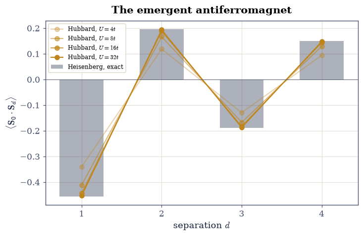The physics follows in three measured acts: double occupancy squeezed from \(1/4\) to \(0.01\) as \(U\) grows; the charge gap opening to \(U - 4t\) while the spin gap stays bounded — the Mott insulator, gapped for charge and soft for spin; and Anderson’s superexchange [And59] — the ground-state spin correlations of the \(U = 32\) Hubbard chain match an independently diagonalized Heisenberg antiferromagnet with \(J = 4t^2/U\) at the percent level, with the deviation falling fourfold per doubling of \(U\), exactly as second-order perturbation theory promises.

Conventions (this notebook). Hopping \(t = 1\) sets the energy unit; chains are periodic unless stated (the dimer is open). Site occupations are bit masks (bit \(i\) set \(=\) orbital \(i\) occupied), one integer per spin species, with the orbital ordering fixed once: all spin-up modes before all spin-down. Fermionic signs are Jordan–Wigner parities computed by int.bit_count of the mask below the acted-on bit. Sector bases are built with itertools.combinations, Hamiltonians as scipy.sparse matrices, ground states by eigsh(k=1, which="SA") (dense numpy.linalg.eigh where the sector is small).

How to read the checks. Each exercise closes with a validate call against an independent fact: an exact anticommutator, a closed-form eigenvalue, a Bethe-ansatz benchmark, a second-order scaling law. A ✓ is strong evidence; a ✗ is a prompt to locate the discrepancy, not an automatic verdict.

Scope. The one-band, one-dimensional, nearest-neighbor Hubbard model at and near half filling, by exact diagonalization. Doped chains, higher dimensions (where the model is believed to hold cuprate superconductivity’s secrets, and is not solved), and the quantum Monte Carlo and DMRG methods that reach them are surveyed in Martin, Reining, and Ceperley [MRC16] Ch. 3 and Vanderbilt-adjacent reviews; the spectral-function view of this same model is §8.14’s business.

Theory in brief

From Wannier orbitals to two parameters

Expand the field operators of §7.23 in a basis of localized Wannier orbitals \(w_i\) and the full interacting Hamiltonian becomes hoppings \(t_{ij}\) plus a four-index Coulomb tensor \(U_{ijkl}\). Hubbard’s cut [Hub63]: for well-localized orbitals the on-site element \(U_{iiii} \equiv U\) dwarfs all others (neighboring-orbital repulsion is screened; exchange is smaller still), and \(t_{ij}\) beyond nearest neighbors decays exponentially (§8.12 measured that decay). What survives is

(903)\[\hat H \;=\; -t \sum_{\langle ij\rangle\sigma} \left(\hat c^\dagger_{i\sigma}\hat c_{j\sigma} + \text{h.c.}\right) \;+\; U \sum_i \hat n_{i\uparrow}\hat n_{i\downarrow} ,\]

the minimal Hamiltonian in which kinetic delocalization and local repulsion compete. At \(U = 0\) it is the tight-binding chain of §8.9, bandwidth \(4t\); at \(t = 0\) each site holds \(0\), \(1\) (\(E = 0\)), or \(2\) (\(E = U\)) electrons and half filling puts exactly one electron per site: an insulator with no kinetic energy at all. The interesting physics is the war between the limits, and the half-filled chain fights it at every \(U\).

The dimer: the model’s hydrogen molecule

Two sites, one electron of each spin, \(S_z = 0\): a four-state problem. In the basis \(\{|\!\uparrow,\downarrow\rangle, |\!\downarrow,\uparrow \rangle, |\!\uparrow\downarrow, 0\rangle, |0, \uparrow\downarrow\rangle\}\) the Hamiltonian is a \(4\times4\) matrix whose singlet sector gives the closed-form ground state

(904)\[E_0 \;=\; \frac{U - \sqrt{U^2 + 16\,t^2}}{2} \;\;\xrightarrow{\;U \gg t\;}\;\; -\,\frac{4t^2}{U} :\]

at large \(U\) the covalent bond gives way to superexchange [And59] — the two spins can no longer share a site, but a virtual double occupation (cost \(U\), amplitude \(t\), twice) still lowers the singlet by \(4t^2/U\) while leaving the triplet untouched. Antiferromagnetism without any magnetic interaction in the Hamiltonian.

The Mott insulator, and the effective spin model

At half filling the charge gap \(\Delta_c = E_0(N{+}1) + E_0(N{-}1) - 2E_0(N)\) — the cost of moving one electron across the system, §8.8’s gap, now for an interacting Hamiltonian — opens for any \(U > 0\) in one dimension (Lieb–Wu [LW68]) and approaches \(U - 4t\) at strong coupling: adding an electron costs the repulsion \(U\), minus the \(4t\) a doubly-occupied site recovers by delocalizing. The spin sector pays no such toll: flipping spins moves no charge, so the spin gap stays of order \(J\) and vanishes as \(L \to \infty\). One material, two energy scales. The surviving low-energy physics is spins only: second-order perturbation theory in \(t/U\) (each neighboring pair enacting the dimer’s virtual hop) maps the half-filled model onto the Heisenberg antiferromagnet

(905)\[\hat H_{\mathrm{eff}} \;=\; J \sum_{\langle ij\rangle} \left(\hat{\mathbf S}_i \cdot \hat{\mathbf S}_j - \tfrac14\right), \qquad J = \frac{4t^2}{U},\]

with corrections entering at relative order \((t/U)^2\). Exercise 6 tests the map where it can be tested: same sizes, both models solved exactly, correlation functions side by side.

Setup

Data and instruments: the hopping unit, the Jordan–Wigner parity of §7.23 restated in bit arithmetic, a basis enumerator, and a ground-state solver wrapper. The notebook’s own machinery — the fermionic operators and the sector Hamiltonian itself — you build in Exercises 1 and 2.

The Setup below holds this notebook’s data and instruments — nothing you are asked to build. It is collapsed so the building stays yours; expand it whenever you want the details.

Show code cell source

Hide code cell source

from itertools import combinations

import numpy as np
import matplotlib.pyplot as plt
from scipy.sparse import lil_matrix
from scipy.sparse.linalg import eigsh

from ecp import validate

INK, AMBER, SOFT = "#16213e", "#c0851a", "#46506b"

T_HOP = 1.0  # data: the hopping integral — the energy unit throughout


# built from scratch in §7.23 (jw_ops, the string of Z's, unit-tested by the
# anticommutator table); restated here in bit arithmetic as an instrument.
def jw_sign(mask, i):
    """Jordan-Wigner sign (-1)^(number of occupied modes below bit i).

    The fermionic sign an operator acting on mode i picks up from
    anticommuting past every occupied mode of lower index.

    Parameters
    ----------
    mask : int
        Occupation bit mask.
    i : int
        Mode index being acted on.

    Returns
    -------
    float
        +1.0 or -1.0.
    """
    return -1.0 if (mask & ((1 << i) - 1)).bit_count() & 1 else 1.0


# instrument: combinatorial plumbing — enumerating fixed-occupation bit
# masks is bookkeeping, not the lesson of any exercise here.
def basis_masks(n_modes, n_occ):
    """All bit masks of n_modes bits with exactly n_occ bits set.

    Parameters
    ----------
    n_modes : int
        Number of orbitals (bits).
    n_occ : int
        Number of occupied orbitals.

    Returns
    -------
    list of int
        The masks, in the canonical combinations order.
    """
    return [sum(1 << i for i in combo) for combo in combinations(range(n_modes), n_occ)]


# instrument: a solver dispatch wrapper (dense below dimension 200, sparse
# Lanczos with a deterministic start vector above) — plumbing, not the
# lesson. It diagonalizes whatever `hubbard_sector` is bound to when it
# runs: the one you build in Exercise 2 (Python looks the name up at call
# time, not at definition time).
def ground_state(n_sites, n_up, n_dn, u_int, pbc=True):
    """Ground energy and vector of a Hubbard sector.

    Uses sparse Lanczos (eigsh, which="SA") for sectors above dimension
    200 and dense numpy.linalg.eigh below.

    Parameters
    ----------
    n_sites, n_up, n_dn : int
        Chain length and electron numbers.
    u_int : float
        On-site repulsion.
    pbc : bool, optional
        Boundary condition.

    Returns
    -------
    tuple
        (E0, ground vector, up masks, down masks).
    """
    ham, ups, dns = hubbard_sector(n_sites, n_up, n_dn, u_int, pbc)
    if ham.shape[0] <= 200:
        vals, vecs = np.linalg.eigh(ham.toarray())
        return float(vals[0]), vecs[:, 0], ups, dns
    # fixed start vector: the U = 0 sector has an open-shell ground-state
    # degeneracy (the k = +-pi/2 levels sit at zero energy), and a
    # symmetric, deterministic v0 selects the same symmetric member on
    # every run instead of whatever Lanczos's random start lands on
    vals, vecs = eigsh(ham, k=1, which="SA", v0=np.ones(ham.shape[0]))
    return float(vals[0]), vecs[:, 0], ups, dns

Exercise 1 — The operators, certified at zero

Everything downstream rests on getting fermionic signs right, so the first exercise builds \(\hat c_i\) as an explicit matrix and checks the algebra — not to a tolerance, but exactly, because Jordan–Wigner signs are integer arithmetic.

Part a) On the \(2^3\)-dimensional Fock space of three spinless modes, build the annihilation matrices: \(\hat c_i\) maps the basis state with mask \(s\) (bit \(i\) set) to the state with mask \(s \oplus 2^i\), weighted by the Jordan–Wigner parity jw_sign(s, i) (§7.23’s convention, now executable).

Part b) Verify the full algebra with numpy matrix products: all nine \(\{\hat c_i, \hat c^\dagger_j\} = \delta_{ij}\mathbb{1}\) and all nine \(\{\hat c_i, \hat c_j\} = 0\), with the maximum absolute deviation equal to \(0.0\) — floating point can represent these signs exactly, so any nonzero deviation means a sign error, full stop. Confirm also that dropping the string (using \(+1\) in place of the parity) breaks the \(i \neq j\) anticommutators: the string is load-bearing.

max |{c_i, cdag_j} - delta_ij| over 9 pairs: 0.0
max |{c_i, c_j}| over 9 pairs:            0.0
without the string: max |{c_i, c_j}| (i != j) = 2.0  (bosons in disguise)

Validation 1 — the algebra is exact, and the string is necessary

Zero means zero here: both anticommutator families at machine-exact \(0.0\), and the string-free counterfeit failing at \(O(1)\).

✓  all 18 anticommutators exact to the last bit   [deviations 0.0, 0.0]
✓  dropping the Jordan-Wigner string breaks the algebra   [max violation 2.0]

True

Exercise 2 — The Hubbard dimer, exactly

The model’s hydrogen molecule, solved both ways — by machinery you must first build.

Part a) Write hubbard_sector(n_sites, n_up, n_dn, u_int, pbc=True), the sparse Hubbard Hamiltonian Eq. 903 in the fixed \((N_\uparrow, N_\downarrow)\) sector: basis states as the product of an up-spin mask and a down-spin mask (flattened as \(a \cdot D_\downarrow + b\)), the interaction diagonal (\(U\) per doubly occupied site), and hopping within each spin species carrying the Jordan–Wigner parity of the bits strictly between the two sites — the boundary bond of a periodic chain crosses the string, so its sign counts every mode in between, which is precisely the subtlety Exercise 1 certified in miniature. Write this one yourself — the implementation is the lesson.

Part b) Certify it on the dimer, whose answer Eq. 904 already gives in closed form: solve the two-site, one-up-one-down system (open boundary) via the Setup’s ground_state — which now drives your machinery — at \(U = 0, 1, 4, 8, 20\), and match the closed form to \(10^{-15}\), five for five.

Part c) Extract the double occupancy \(d = \langle \hat n_{i\uparrow}\hat n_{i\downarrow}\rangle\) per site from the ground vector. At \(U = 0\) the two electrons ignore each other and \(d = 1/4\) exactly (each site’s up and down occupations independent, each \(1/2\)); repulsion strangles it.

Part d) Watch superexchange emerge: at \(U = 10, 20, 40\) compare \(E_0\) with \(-4t^2/U\) — the ratio must walk monotonically to \(1\) (\(0.963\), \(0.990\), \(0.9975\): the second-order correction \(4t^2/U^2\) dying as promised), the singlet’s virtual-hopping reward.

U =    0: ED -2.000000000000   closed form -2.000000000000
U =    1: ED -1.561552812809   closed form -1.561552812809
U =    4: ED -0.828427124746   closed form -0.828427124746
U =    8: ED -0.472135955000   closed form -0.472135955000
U =   20: ED -0.198039027186   closed form -0.198039027186
worst deviation over the five: 3.7e-15
double occupancy at U = 0: 0.2500000000  (exact 1/4)
E0 / (-4t^2/U) at U = 10, 20, 40: 0.9629, 0.9902, 0.9975

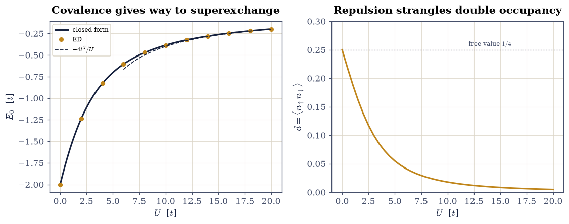
Fig. 809 The Hubbard dimer, exactly. Left: the ground energy against \(U\) — exact diagonalization (amber points) on the closed form \((U - \sqrt{U^2 + 16t^2})/2\) (ink), which starts out as the covalent bond \(-2t + U/2\) at weak coupling and lands on Anderson’s superexchange \(-4t^2/U\) (dashed) at strong. Right: double occupancy strangled from its free value \(1/4\) (dotted) toward zero as \(U\) grows — the electrons still bond, but they no longer share a room.

Validation 2 — the dimer knows its closed form

Five exact energies at \(10^{-14}\), the free-electron \(d = 1/4\), and the superexchange ratio marching monotonically to \(1\).

✓  dimer ED = closed form at U = 0, 1, 4, 8, 20   [worst |dE| = 3.7e-15]
✓  U = 0 double occupancy = 1/4   [got 0.25 vs expected 0.25 (rtol=1e-12, atol=1e-09)]
✓  E0 -> -4t^2/U monotonically (0.3% by U = 40t)   [ratios 0.9629 -> 0.9975]

True

Exercise 3 — Eight sites: the sector, benchmarked twice

Now the machinery earns its keep: the half-filled \(L = 8\) periodic chain.

Part a) Count before computing: the \(S_z = 0\), \(N = 8\) sector is \(\binom{8}{4}^2 = 4900\)-dimensional (the full Fock space is \(4^8 = 65{,}536\); symmetry buys a factor of \(13\)). Build the sector Hamiltonian with the hubbard_sector you wrote in Exercise 2 and confirm dimension and Hermiticity (scipy.sparse max asymmetry, exactly \(0\)).

Part b) Benchmark against the two ends of the coupling axis. At \(U = 0\) the periodic tight-binding levels \(-2t\cos(2\pi m/8)\) filled with four electrons per spin give \(E_0/L = -(1 + \sqrt2)/2 = -1.20711\) exactly (the \(k = \pm\pi/2\) levels sit at zero energy, so the open-shell degeneracy costs nothing); eigsh must land on it at \(10^{-9}\). At \(U = 4\) compare with the exact infinite-chain Bethe-ansatz energy of Lieb and Wu [LW68], \(-0.573729\) per site: eight sites land at \(-0.575441\), within \(0.3\%\) — exact diagonalization touching an exact solution.

sector dimension: 4900  (C(8,4)^2 = 4900); full Fock space 4^8 = 65536
max |H - H^T|: 0.0
U = 0: E0 = -9.6568542495   closed form 8 x -(1+sqrt(2))/2 = -9.6568542495

U = 4: E0/L = -0.575441   Lieb-Wu (L -> inf) -0.573729   finite-size deviation 0.30%

Validation 3 — counted, symmetric, and twice benchmarked

Dimension \(4900\), symmetry exact, the \(U = 0\) closed form at \(10^{-9}\), and Lieb–Wu within half a percent from eight sites.

✓  sector dimension 4900 and H exactly symmetric   [dim 4900, asym 0.0]
✓  U = 0 energy = -(1+sqrt(2))/2 per site   [got -9.65685 vs expected -9.65685 (rtol=1e-09, atol=1e-09)]
✓  eight sites within 0.5% of the infinite-chain Bethe ansatz (U = 4)   [deviation 0.30%]

True

Exercise 4 — The crossover: kinetic energy pays the repulsion’s toll

With the machinery certified, sweep the war between the limits.

Part a) For \(U = 0\) to \(16\), compute \(E_0/L\) and the double occupancy of the half-filled chain. Both must fall monotonically: energy because \(U\) only adds a positive diagonal, double occupancy because that is how the ground state dodges the toll — from exactly \(1/4\) at \(U = 0\) (the uncorrelated value; the free chain’s open-shell degeneracy is resolved deterministically by the fixed Lanczos start vector) to \(0.011\) at \(U = 16\), a \(96\%\) eviction.

Part b) The eviction is the Mott localization in slow motion: plot both curves, and against the \(E_0/L\) curve mark the two asymptotes it interpolates — the free value \(-(1+\sqrt2)/2\) and the superexchange energy per site of the effective Heisenberg model (Exercise 6’s \(J(E_{\mathrm{Heis}} - L/4)/L\) with \(J = 4t^2/U\)).

U =    0: E0/L = -1.207107   d = 0.25000
U =    1: E0/L = -0.994041   d = 0.19234
U =    2: E0/L = -0.821024   d = 0.15449
U =    3: E0/L = -0.683325   d = 0.12183
U =    4: E0/L = -0.575441   d = 0.09493
U =    6: E0/L = -0.426097   d = 0.05783
U =    8: E0/L = -0.333268   d = 0.03702
U =   12: E0/L = -0.229311   d = 0.01812
U =   16: E0/L = -0.173958   d = 0.01055

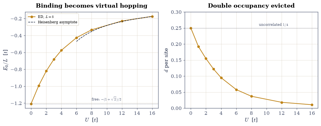
Fig. 810 The half-filled chain’s crossover, measured. Left: ground energy per site rising from the free-electron \(-(1+\sqrt{2})/2\) (dotted) toward zero, hugging the superexchange asymptote \(J(E_{\mathrm{Heis}}/L - 1/4)\) (dashed) beyond \(U \approx 8t\): by \(U = 16t\) the remaining binding energy is pure virtual hopping. Right: double occupancy evicted from the uncorrelated \(1/4\) at \(U = 0\) to \(0.011\) at \(U = 16\) — the ground state buys its way out of the repulsion by localizing one electron per site, which is precisely what a Mott insulator is.

Validation 4 — both monotone, and quantitatively evicted

Energy and double occupancy strictly falling across the nine couplings; \(d(U{=}16) \approx 0.011\), and the large-\(U\) energy within \(2\%\) of the Heisenberg asymptote.

✓  E0/L rises and d falls monotonically with U   [d: 0.250 -> 0.011]
✓  d(U = 16) (96% eviction)   [got 0.01055 vs expected 0.0106 (rtol=0.05, atol=1e-09)]
✓  E0/L(U = 16) on the superexchange asymptote   [got -0.173958 vs expected -0.176597 (rtol=0.02, atol=1e-09)]

True

Exercise 5 — The Mott gap: charge pays, spin does not

§7.12’s rule — half-filled band, therefore metal — meets its counterexample.

Part a) Compute the charge gap \(\Delta_c = E_0(5,4) + E_0(3,4) - 2E_0(4,4)\) (add an electron, remove one; particle–hole symmetry makes the two sectors’ costs equal) at \(U = 2, 4, 8, 16\): it grows from \(0.80\) through \(2.01\) and \(5.19\) to \(12.66\), closing on the strong-coupling law \(U - 4t\) (deviation \(0.65t\) at \(U = 16\) and shrinking).

Part b) Compute the spin gap \(\Delta_s = E_0(5,3) - E_0(4,4)\) — the cost of one spin flip, no charge moved. It stays below \(0.35t\) at every coupling (and vanishes as \(L \to \infty\): the Bethe-ansatz spin sector is gapless). One system, two prices: this hierarchy is the Mott insulator — insulating for charge transport, alive with spin dynamics. A free-electron system cannot do this: at \(U = 0\) both gaps are finite- size artifacts of the same magnitude.

U =    2: charge gap  0.7998   spin gap 0.1585   ratio    5.0
U =    4: charge gap  2.0122   spin gap 0.3035   ratio    6.6
U =    8: charge gap  5.1858   spin gap 0.2396   ratio   21.6
U =   16: charge gap 12.6552   spin gap 0.1284   ratio   98.5

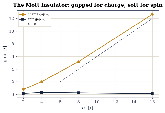
Fig. 811 One chain, two prices. The charge gap (amber: add plus remove an electron) opens with \(U\) and closes on the strong-coupling law \(U - 4t\) (dashed): by \(U = 16t\) moving charge across the half-filled chain costs \(12.7t\). The spin gap (ink: flip one spin, move no charge) never exceeds \(0.35t\) and is headed for zero at infinite length. The band picture of §7.12 has no vocabulary for this split — a Mott insulator is gapped and gapless at the same time, depending on what you ask it to transport.

Validation 5 — the hierarchy, quantified

Charge gap strictly growing and within \(0.7t\) of \(U - 4t\) at \(U = 16\); spin gap bounded by \(0.35t\) throughout; a factor \(\geq 20\) between the two sectors at strong coupling.

✓  charge gap grows monotonically with U   [0.80 -> 12.66]
✓  charge gap -> U - 4t   [got 12.6552 vs expected 12 (rtol=1e-06, atol=0.7)]
✓  spin gap bounded (gapless sector in disguise)   [max 0.304 t]
✓  charge/spin price ratio exceeds 20 at U = 16   [ratio 99]

True

Exercise 6 — Verdict: the hidden Heisenberg model

Equation Eq. 905 claims that at strong coupling the Hubbard chain is a spin chain. Both sides can be diagonalized exactly at \(L = 8\); nothing needs to be taken on faith.

Part a) Build and solve the \(L = 8\) periodic Heisenberg antiferromagnet (\(J = 1\)) in its own \(S_z = 0\) basis (\(\binom{8}{4} = 70\) states): ground energy \(E_{\mathrm{Heis}} = -3.651093\) and the ground-state correlations \(\langle\mathbf S_0\cdot\mathbf S_d\rangle\) for \(d = 1\)–\(4\), sign-alternating (antiferromagnetic) with slowly decaying magnitude — the correlations that become Bethe’s famous critical spin chain at \(L \to \infty\).

Part b) Measure the same correlator in the Hubbard ground state (\(\hat{\mathbf S}_i\) built from the fermionic operators) at \(U = 4, 8, 16, 32\) and set the two spin chains side by side. The match must improve as \((t/U)^2\): maximum relative deviation (over the four distances) \(39\%\) at \(U = 4\) falling to \(1.1\%\) at \(U = 32\), roughly fourfold per doubling. Check the energies too: \(E_0^{\mathrm{Hub}}\) against \(J(E_{\mathrm{Heis}} - L/4)\) at \(U = 32\), within half a percent.

Part c) Print the verdict table — \(U\), \(E_0/L\), \(d\), \(\Delta_c\), \(\Delta_s\), and the Heisenberg deviation — and read it as one story: repulsion evicts double occupancy, the eviction gaps the charge sector, and what survives below the gap is an antiferromagnet no term of Eq. 903 asked for.

Heisenberg L = 8: E0 = -3.651093
  <S0.Sd>, d = 1..4: -0.45639, +0.19578, -0.18895, +0.14912

U =    4: -0.33996, +0.11858, -0.12945, +0.09403   max dev  39.4%

U =    8: -0.41112, +0.16651, -0.16701, +0.12877   max dev  14.9%

U =   16: -0.44357, +0.18767, -0.18298, +0.14357   max dev   4.1%

U =   32: -0.45308, +0.19370, -0.18743, +0.14771   max dev   1.1%

E0(U = 32) = -0.70370   J(E_Heis - L/4) = -0.70639   dev 0.38%

--- Verdict: how a metal becomes an antiferromagnetic insulator ---
   U      E0/L    docc  ch.gap  sp.gap  Heis.dev
   4   -0.5754  0.0949   2.012   0.304     39.4%
   8   -0.3333  0.0370   5.186   0.240     14.9%
  16   -0.1740  0.0106  12.655   0.128      4.1%
  32       nan     nan     nan     nan      1.1%

Fig. 812 Anderson’s superexchange, verified at the percent level. Ground-state spin correlations \(\langle\mathbf{S}_0\cdot\mathbf{S}_d\rangle\) of the half-filled Hubbard chain at \(U/t = 4, 8, 16, 32\) (amber, deepening) against the exactly diagonalized \(L = 8\) Heisenberg antiferromagnet (ink bars) — the model Eq. 905 says they must become. The alternating signs are there at every coupling; the magnitudes converge onto the Heisenberg values as \((t/U)^2\), from \(39\%\) off at \(U = 4t\) (worst of the four distances) to \(1.1\%\) at \(U = 32t\). The Hubbard Hamiltonian contains no spin coupling; the antiferromagnet is entirely emergent.

Validation 6 — superexchange at the percent level

Heisenberg ground energy against its known value; alternating signs at every coupling; the worst-of-four deviation falling as second order demands; and the energy map closing within half a percent at \(U = 32\).

✓  L = 8 Heisenberg ground energy   [got -3.65109 vs expected -3.65109 (rtol=1e-06, atol=1e-09)]
✓  antiferromagnetic sign alternation at every U   [signs -,+,-,+ for d = 1..4]
✓  Heisenberg deviation falls monotonically to ~1% at U = 32   [39% -> 1.1%]
✓  deviation shrinks fourfold per doubling of U (second order in t/U)   [ratio 3.9]
✓  E0(U = 32) = J(E_Heis - L/4) within 0.5%   [got -0.703699 vs expected -0.706387 (rtol=0.005, atol=1e-09)]

True

With your assistant

Away from half filling the Mott insulator becomes one of the strangest metals known: in one dimension the electron falls apart into separate spin and charge excitations. A first look is within your reach: have your assistant compute the ground energy of the \(L = 8\), \(U = 8\) chain with \(N = 8, 7, 6\) electrons (\(S_z = 0\) or \(\pm\tfrac12\) sectors) and form the chemical potentials \(\mu^+ = E_0(N{+}1) - E_0(N)\) and \(\mu^- = E_0(N) - E_0(N{-}1)\) at \(N = 7\). Then run the check that is yours alone: at \(N = 7\) (doped) the two chemical potentials must differ by far less than the half-filled charge gap — numpy.isclose of \(\mu^+ - \mu^-\) against \(0\) with atol a tenth of Exercise 5’s \(\Delta_c(U{=}8)\) — the doped chain conducts, the half-filled one cannot. The check is yours.

Notebook summary

Movement IV opened with the band picture’s minimal enemy: two terms, one competition. The fermionic algebra was built as matrices and certified at exactly zero error — 18 anticommutators, integer arithmetic, no tolerance — with the Jordan–Wigner string shown load-bearing by breaking it. The dimer matched its closed form \((U - \sqrt{U^2 + 16t^2})/2\) at \(10^{-15}\) five times over and handed us superexchange in miniature (ratio to \(-4t^2/U\) walking \(0.963 \to 0.9975\) from \(U = 10\) to \(40\)). Eight periodic sites at half filling — a 4900-dimensional sector, eigsh, a tenth of a second — hit the \(U = 0\) closed form \(-(1+\sqrt2)/2\) at \(10^{-10}\) and Lieb–Wu’s infinite-chain Bethe ansatz within \(0.3\%\). Then the physics: double occupancy evicted from \(1/4\) to \(0.011\); the charge gap climbing \(0.80 \to 12.66\) onto the \(U - 4t\) law while the spin gap idled below \(0.35t\) — a system insulating for charge and gapless for spin, which no independent-electron theory of this volume can produce; and the buried punchline, Anderson’s superexchange, verified by diagonalizing the Heisenberg chain the Hubbard model is supposed to become and watching four correlation functions converge onto it as \((t/U)^2\) — worst-distance deviations \(39\%\), \(15\%\), \(4\%\), \(1.1\%\) — with the ground energies agreeing through \(J = 4t^2/U\) to \(0.4\%\). An antiferromagnet emerged from a Hamiltonian containing no spin coupling whatsoever.

Outlook

• Everything here was energies and equal-time correlators. The dynamics — what happens when one electron is injected or removed, the spectral function that photoemission actually measures — needs the Lehmann machinery of §8.14, where this same \(N \pm 1\) sector arithmetic becomes \(A(k, \omega)\) and the GW approximation is tested against exactly these chains.

• The \(4900\)-dimensional sector was comfortable; \(L = 16\) is \(165\) million. The exponential wall is real, and the methods that negotiate it — quantum Monte Carlo (§7.21 grown up), DMRG, embedding — define modern many-body practice; Martin, Reining, and Ceperley [MRC16] surveys the field (Ch. 23–25 for the stochastic methods).

• In two dimensions the doped Hubbard model is the leading candidate theory of high-temperature superconductivity — unsolved after four decades. The one-dimensional physics computed here (spin–charge separation, emergent magnetism) is the solved corner of that problem.

[And59] (1,2)

P. W. Anderson. New approach to the theory of superexchange interactions. Physical Review, 115:2–13, 1959.

[Hub63] (1,2)

J. Hubbard. Electron correlations in narrow energy bands. Proceedings of the Royal Society of London A, 276:238–257, 1963. doi:10.1098/rspa.1963.0204.

[LW68] (1,2,3)

Elliott H. Lieb and F. Y. Wu. Absence of Mott transition in an exact solution of the short-range, one-band model in one dimension. Physical Review Letters, 20:1445–1448, 1968.

[MRC16] (1,2)

Richard M. Martin, Lucia Reining, and David M. Ceperley. Interacting Electrons: Theory and Computational Approaches. Cambridge University Press, Cambridge, 2016.

Take this notebook with you

Use the download button (↓) in the toolbar above to save this notebook and run it yourself. The published notebooks ship without worked solutions; if you would like the reference solutions — to teach from or to check your own work — get in touch: hello@ramador.me.