


6.8 Qubits, the Bloch Sphere, and a First Taste of Entanglement#
Notebook overview#
This is the capstone of Movement I, and it does two things. First it gives the qubit its geometry. Everything we have built for a two-level system — superposition, measurement, uncertainty, dynamics — turns out to fit on the surface of a single sphere, and once that picture is in hand, the whole movement can be seen at a glance. A qubit’s physical state, a ray in \(\mathbb{C}^2\), is a point on the Bloch sphere; its coordinates are the Pauli expectation values; orthogonal states sit at opposite poles; and a unitary operation is a rotation — the Larmor precession of §6.7 made literal, a Bloch vector spinning about the field axis.
Then the notebook takes the first real step beyond a single particle, and meets the one phenomenon that has no classical shadow at all. Two qubits live in the tensor product \(\mathbb{C}^2\otimes \mathbb{C}^2\), and most of the states there are not products of individual states: they are entangled. The canonical example is the Bell state \((|00\rangle+|11\rangle)/\sqrt2\), and its signature is startling — the whole is a perfectly definite (pure) state, yet each part, taken alone, is maximally uncertain. The information is not in the pieces; it is entirely in the correlations between them. We diagnose this precisely (the Schmidt rank, the reduced state’s mixedness) and end on the puzzle that breaks classical realism: correlations perfect in two incompatible bases, which no pre-assigned values could ever reproduce.
As in every Volume VI notebook, each exercise opens with a crystal-clear statement and enumerated parts, each naming the exact operation — the Bloch vector from Pauli expectation values, numpy.kron
for the tensor product, numpy.linalg.svd for the Schmidt decomposition, a reshape-and-contract for
the reduced density matrix, and numpy.linalg.eigvalsh for its spectrum.
A boundary, stated up front. Entanglement forces us to meet a new object — the reduced density matrix \(\rho_A=\mathrm{Tr}_B|\psi\rangle\langle\psi|\), the state of part of an entangled pair, together with its purity \(\mathrm{Tr}(\rho^2)\) and entanglement entropy \(S=-\mathrm{Tr}(\rho \log_2\rho)\) (the 5.x entropy of the reduced state). We use it here only as the diagnostic of entanglement; the general density-matrix formalism — mixed states from classical ignorance, the full theory — is §6.26. Likewise the Bell correlations here are a taste; the quantitative Bell-inequality violation is §6.25.
How to read the checks. Each exercise closes with a
validatecall: the Bloch map and unit purity of a pure state; global-phase invariance; orthogonal states antipodal and precession a rotation; the tensor-product structure; the Bell state’s Schmidt rank 2 versus a product’s rank 1; the Bell reduced state maximally mixed (purity \(\tfrac12\), \(S=1\) bit); and the perfect Bell correlations with random marginals. A ✓ is strong evidence; a ✗ is a prompt to locate the discrepancy.Conventions and scope. A qubit is parametrized as \(|\psi\rangle=\cos\tfrac\theta2|0\rangle+ e^{i\varphi}\sin\tfrac\theta2|1\rangle\); in
numpy.kron(a, b)the first factor is qubit \(A\), so \(|q_Aq_B\rangle\) is index \(2q_A+q_B\). The Pauli matrices are those of §6.6. Mixed states (inside the sphere) and the general density operator are §6.26; Bell’s inequality is §6.25; wave mechanics (the same formalism in infinite dimensions) opens Movement II in §6.9. See Nielsen & Chuang; Sakurai & Napolitano; and Notebooks §6.1 (rays, global phase), §6.6 (Pauli expectations), §6.7 (precession), 5.x (entropy).
Theory in brief#
The Bloch sphere#
Any qubit state, with its global phase removed, is
a point on the unit sphere whose Cartesian coordinates are the Pauli expectation values (the Bloch vector). The global phase of §6.1 is exactly what is quotiented away — the ray becomes a point — and a pure state has \(|\mathbf b|=1\). Poles: \(|0\rangle\) (north), \(|1\rangle\) (south); equator: \(|{\pm}\rangle\), \(|{\pm}i\rangle\).
Geometry of states and evolution#
The Bloch map turns Hilbert-space relations into spherical geometry: a short computation in the half-angle parametrization gives \(|\langle\phi|\psi\rangle|^2=\tfrac12(1+\mathbf b_\phi\cdot\mathbf b_\psi)\) for pure states (Nielsen & Chuang develop the full dictionary), so overlaps become angles and overlap-preserving unitaries become rotations:
Orthogonal states are antipodal (note the factor of two between the Hilbert-space angle and the Bloch angle — the spin-\(\tfrac12\) double cover), a unitary is a rotation, and the Larmor precession of §6.7 is literally the Bloch vector rotating about the field at the Larmor frequency. (Mixed states, §6.26, live inside the sphere.)
The tensor product: composite systems#
Two qubits live in the tensor product,
A product (separable) state is \(|a\rangle\otimes|b\rangle\); a single-qubit observable is \(A\otimes I\). This is how quantum mechanics describes more than one particle.
Entanglement#
Some two-qubit states are not products,
The Schmidt decomposition diagnoses it: reshape the 4-vector to a \(2\times2\) matrix and take its
singular values (numpy.linalg.svd). A product state has Schmidt rank 1 (one nonzero singular
value); an entangled state has rank \(\ge2\). The Bell state has rank 2 with equal coefficients.
The signature: the reduced state is mixed#
For an entangled pure state, the reduced density matrix of one qubit is mixed,
maximally mixed — even though the whole is pure. A product state instead gives a pure reduced state (purity 1, \(S=0\)). The whole is sharp, each part maximally uncertain: the information is in the correlations, not the pieces. (This is the first density matrix; the general theory is §6.26.)
Bell correlations — the taste#
In the Bell state the two qubits are perfectly correlated in two incompatible bases while each alone is random,
Correlations this strong in incompatible bases cannot come from pre-assigned (local hidden-variable) values — the puzzle Bell’s inequality (§6.25) makes quantitative.
Setup#
The data are the series palette, the Pauli matrices and the \(2\times2\) identity of
§6.6, the index conventions (\(\hbar=1\); numpy.kron(a, b) puts qubit \(A\)
first), and the given half-angle parametrization qubit of Eq. 532 — the specimen states,
not machinery. The instruments are the expectation value \(\langle\psi|A|\psi\rangle\) of
§6.5, the two mixedness meters purity and entanglement_entropy that read
numbers off a density matrix, and the Bloch-sphere drawing frame. This notebook’s own machinery is
not here: you write the Bloch map bloch_vector in Exercise 1, the Schmidt coefficients
schmidt in Exercise 4, and the partial trace reduced_density_matrix in Exercise 6. No
randomness appears anywhere in this notebook.
The Setup below holds this notebook’s data and instruments — nothing you are asked to build. It is collapsed so the building stays yours; expand it whenever you want the details.
Exercise 1 — The Bloch sphere map#
The map at the centre of this notebook sends a qubit state to the triple of its Pauli expectation values, \(\mathbf b=(\langle\sigma_x\rangle,\langle\sigma_y\rangle,\langle\sigma_z\rangle)\) — three numbers, each an expectation of a \(2\times2\) Hermitian matrix, read as Cartesian coordinates. In the half-angle parametrization \(|\psi\rangle=\cos\tfrac\theta2|0\rangle+e^{i\varphi}\sin\tfrac \theta2|1\rangle\) that triple is \((\sin\theta\cos\varphi,\sin\theta\sin\varphi,\cos\theta)\): a point on the unit sphere, with a pure state always on the surface, \(|\mathbf b|=1\) Eq. 532.
Write
bloch_vector(psi), returning the three Pauli expectation values ofpsias a length-3 array (the Setup’sexpectationhelper onSIGMA_X,SIGMA_Y,SIGMA_Z).Build \(|\psi\rangle\) with the
qubithelper for a chosen \((\theta,\varphi)\).Compute its Bloch vector.
Confirm it equals \((\sin\theta\cos\varphi,\sin\theta\sin\varphi,\cos\theta)\) with
numpy.allclose, and that \(|\mathbf b|=1\) (numpy.linalg.norm).Check the special points: \(|0\rangle\to(0,0,1)\), \(|1\rangle\to(0,0,-1)\), \(|{+}\rangle\to(1,0,0)\), \(|{+}i\rangle\to(0,1,0)\). The ray becomes a point.
Bloch vector  = [0.6981 0.588  0.4085]
(sinθcosφ, …) = [0.6981 0.588  0.4085]   (match: True);  |b| = 1.000000
  |0⟩   → [0. 0. 1.]
  |1⟩   → [ 0.  0. -1.]
  |+⟩   → [1. 0. 0.]
  |+i⟩  → [0. 1. 0.]
Validation 1#
✓  the Bloch vector is the triple of Pauli expectation values; a pure qubit is a point on the unit sphere   [max|Δ| = 1.66533e-16 (rtol=1e-12, atol=1e-09)]
✓  a pure state has a unit Bloch vector (it lies on the surface of the sphere)   [got 1 vs expected 1 (rtol=1e-12, atol=1e-09)]
True
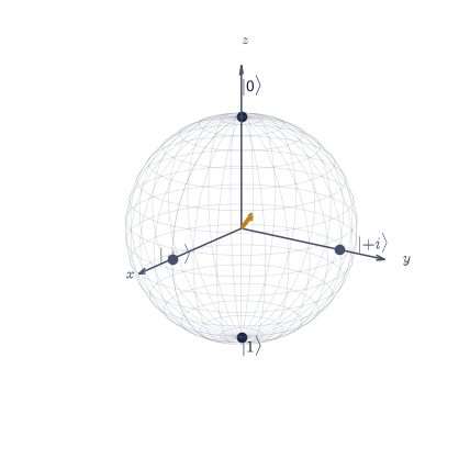
Fig. 525 The Bloch sphere. Every physical state of a single qubit is a point on this unit sphere; its Cartesian coordinates are the Pauli expectation values \((\langle\sigma_x\rangle,\langle\sigma_y\rangle,\langle\sigma_z\rangle)\). The computational basis sits at the poles — \(|0\rangle\) north, \(|1\rangle\) south — and the equator carries the superpositions \(|{\pm}\rangle\) and \(|{\pm}i\rangle\); a generic state (amber) points to \((\theta,\varphi)\). The global phase of §6.1 is exactly what has been quotiented away to turn a ray into a point, and orthogonal states sit at opposite poles. This single picture holds all of Movement I: a measurement is a projection onto an axis, an evolution is a rotation, and (§6.26) a mixed state is a point inside the ball.#
Exercise 2 — Global phase and the sphere#
The global-phase ambiguity of §6.1 is exactly the quotient that turns a state vector into a point: multiplying \(|\psi\rangle\) by \(e^{i\alpha}\) leaves every Pauli expectation — hence the Bloch vector — unchanged, so the sphere is the space of physical states (rays) Eq. 532.
Take a state \(|\psi\rangle\) and the phase-shifted \(e^{i\alpha}|\psi\rangle\) (
numpy.exp(1j*alpha)).Compute both Bloch vectors with the
bloch_vectoryou wrote in Exercise 1.Confirm they are identical (
numpy.allclose).Read the meaning: the Bloch sphere is the set of rays — the “a global phase means nothing” of §6.1 made geometric.
Bloch(|ψ⟩)        = [0.6981 0.588  0.4085]
Bloch(e^(iα)|ψ⟩) = [0.6981 0.588  0.4085]   (identical: True)
→ the global phase is invisible on the sphere: a point is a ray, not a vector.
Validation 2#
✓ a global phase leaves the Bloch point fixed — the sphere is the space of physical states (rays), §6.1 made geometric [max|Δ| = 1.11022e-16 (rtol=1e-12, atol=1e-09)]
True
Exercise 3 — Orthogonality and evolution as geometry#
Two geometric facts turn Hilbert-space relations into pictures on the sphere: orthogonal qubit
states are antipodal, and Larmor precession (§6.7) is literally a rotation of the
Bloch vector about the field axis Eq. 533 — Movement I’s dynamics made visible.
Both are read here with the bloch_vector you wrote in Exercise 1.
Confirm \(|0\rangle\) and \(|1\rangle\) (and another orthogonal pair) map to opposite points, \(\mathbf b_\phi=-\mathbf b_\psi\) — noting the factor of two between the Hilbert-space angle (\(90^\circ\)) and the Bloch angle (\(180^\circ\)), the spin-\(\tfrac12\) double cover.
Evolve \(|{+} \rangle\) under the Larmor Hamiltonian \(H=-\tfrac\omega2\sigma_z\) (§6.7) using the spectral construction.
Compute the Bloch vector versus time.
Confirm it rotates about \(z\) at frequency \(\omega\): \(\mathbf b(t)=(\cos\omega t,-\sin\omega t,0)\), the latitude fixed.
⟨ψ⊥|ψ⟩ = 0.0e+00+0.0e+00j;  Bloch antipodal (b_⊥ = −b_ψ): True
  Hilbert angle 90° ↔ Bloch angle 180° (the spin-½ factor of two)
precession is rotation about z: Bloch(t) = (cos ωt, −sin ωt, 0)?  True
  ⟨σz⟩ (latitude) fixed at 2.2e-16
Validation 3#
✓  orthogonal qubit states are antipodal on the Bloch sphere (the factor-of-two double cover)
✓  Larmor precession is a rotation of the Bloch vector about the field axis at frequency ω   [max|Δ| = 2.22045e-16 (rtol=1e-06, atol=1e-10)]
True
Fig. 526 Precession is rotation, animated. The qubit \(|{+}\rangle\) evolving under \(H=-\tfrac\omega2\sigma_z\) traces its Bloch vector (amber) around the equator at the Larmor frequency \(\omega\), the dotted circle marking the path. This is the same motion as the expectation-value precession of §6.7 — \(\langle S_x\rangle=\tfrac12\cos\omega t\), \(\langle S_y\rangle=-\tfrac12\sin\omega t\) — but now seen for what it geometrically is: a rigid rotation of the sphere about the field axis. Every unitary evolution is such a rotation; the Hamiltonian picks the axis and the rate.#
Exercise 4 — The tensor product and composite systems#
The tensor product is how quantum mechanics describes more than one particle: two qubits live in \(\mathbb{C}^2\otimes\mathbb{C}^2=\mathbb{C}^4\), a product state is \(|a\rangle\otimes|b\rangle\), and a single-qubit observable is \(A\otimes I\) Eq. 534. The four amplitudes of a two-qubit state can equally be read as a \(2\times2\) matrix \(M_{ab}\) (rows = qubit \(A\), columns = qubit \(B\)), and the singular values of that matrix are the Schmidt coefficients Eq. 535 — the tool Exercise 5 turns into the test for entanglement, and the tool that certifies here that a product state really does factorize.
Write
schmidt(state4), which reshapes the length-4 state to the \(2\times2\) amplitude matrix and returns its singular values,numpy.linalg.svd(..., compute_uv=False).Form a product state \(|a\rangle\otimes|b\rangle\) with
numpy.kronand confirm the basis ordering \(\{|00\rangle,|01\rangle,|10\rangle,|11\rangle\}\).Build the single-qubit observables \(\sigma_z\otimes I=\)
numpy.kron(SIGMA_Z, ID2)and \(I\otimes\sigma_z\).Verify that \(\langle\sigma_z\otimes I\rangle\) on \(|a\rangle\otimes|b\rangle\) reports qubit \(A\)’s own \(\langle \sigma_z\rangle\) (the
expectationhelper), and likewise \(I\otimes\sigma_z\) for qubit \(B\).Confirm a product state factorizes: its Schmidt rank, the number of nonzero coefficients, is 1.
⟨σz⊗I⟩ on |a⟩⊗|b⟩ = 0.8253   vs qubit A's own ⟨σz⟩ = 0.8253
⟨I⊗σz⟩ on |a⟩⊗|b⟩ = 0.4536   vs qubit B's own ⟨σz⟩ = 0.4536
product state Schmidt rank = 1   (factorizes)
Validation 4#
✓ two qubits live in the tensor product ℂ²⊗ℂ²; a single-qubit observable A⊗I reports that qubit's own expectation value [max|Δ| = 2.77556e-16 (rtol=1e-12, atol=1e-09)]
True
Exercise 5 — Entanglement and the Schmidt decomposition#
The Schmidt coefficients decide whether a two-qubit state is a product or entangled: the number of nonzero coefficients is the Schmidt rank, and a product state has rank 1 while an entangled state has rank \(\ge2\) Eq. 535. The canonical entangled state is the Bell state \(|\Phi^+\rangle=(|00\rangle+|11\rangle)/\sqrt2\), whose amplitude matrix is \(\tfrac1{\sqrt2}I\) — two equal singular values, and no way to write it as one product.
Build the Bell state \(|\Phi^+\rangle\) as a length-4 amplitude vector.
Take the Schmidt coefficients of the product state of Exercise 4 and of the Bell state, with the
schmidtyou wrote in Exercise 4.Count the nonzero coefficients of each — rank 1 (coefficients \(1,0\)) versus rank 2 (equal coefficients \(1/\sqrt2,1/\sqrt2\)). Entanglement is non-factorizability.
product state |a⟩⊗|b⟩:  Schmidt coefficients [1. 0.]  → rank 1 (separable)
Bell state |Φ+⟩:        Schmidt coefficients [0.7071 0.7071]  → rank 2 (entangled)
Validation 5#
✓ an entangled state cannot be factored: the product state has Schmidt rank 1, the Bell state rank 2
True
Exercise 6 — The reduced density matrix: the part is mixed#
The signature of entanglement is that the reduced state of a part is mixed even though the whole is pure: for the Bell state \(\rho_A\) is maximally mixed (purity \(\tfrac12\), entanglement entropy \(1\) bit), while a product state gives a pure reduced state Eq. 536. Tracing out qubit \(B\) is the same reshape as the Schmidt decomposition, one contraction further: read the four amplitudes as the matrix \(M_{ab}\) (rows = qubit \(A\), columns = qubit \(B\)) and sum over the \(B\) index against the conjugate, which is the matrix product \(\rho_A=MM^{\dagger}\). Getting the index order right is the whole of it — contract the wrong index and you get qubit \(B\) instead.
Write
reduced_density_matrix(state4), returning \(\rho_A=\mathrm{Tr}_B|\psi\rangle\langle\psi|\) as the \(2\times2\) matrix \(MM^{\dagger}\). Write this one yourself — the implementation is the lesson.Compute its eigenvalues (
numpy.linalg.eigvalsh), purity \(\mathrm{Tr}(\rho_A^2)\) (thepurityhelper), and entanglement entropy \(S=-\sum\lambda\log_2\lambda\) (theentanglement_entropyhelper).For the product state find a pure \(\rho_A\) (eigenvalues \(0,1\); purity \(1\); \(S=0\)).
For the Bell state find a maximally mixed \(\rho_A\) (eigenvalues \(\tfrac12,\tfrac12\); purity \(\tfrac12\); \(S=1\) bit) — its Bloch vector is the origin. The whole is sharp, the parts blurred; the information is in the correlations.
product reduced ρ_A:  eigenvalues [0. 1.], purity 1.0000, S = 0.0000 bit  (pure)
Bell reduced ρ_A:     eigenvalues [0.5 0.5], purity 0.5000, S = 1.0000 bit  (maximally mixed)
Bell reduced Bloch vector = [0. 0. 0.]   (the origin: maximally mixed)
Validation 6#
✓  for the Bell state the reduced single-qubit state is maximally mixed (purity ½, entanglement entropy 1 bit) — the part is mixed though the whole is pure   [max|Δ| = 2.22045e-16 (rtol=1e-10, atol=1e-09)]
✓  for a product state the reduced state is pure (purity 1, entropy 0) — no entanglement   [max|Δ| = 5.55112e-16 (rtol=1e-06, atol=1e-10)]
True
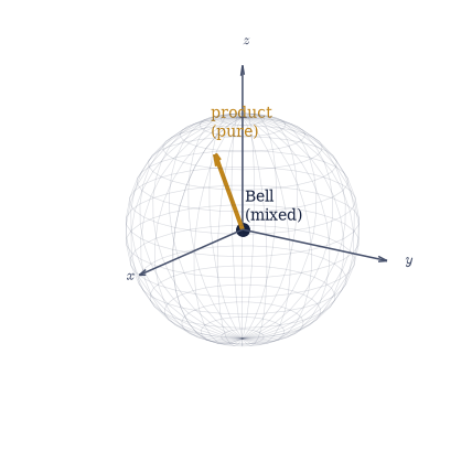
Fig. 527 The part of an entangled whole is blurred. Two single-qubit reduced states on the Bloch ball. For a product state (amber) the reduced qubit is itself pure — a unit Bloch vector on the surface, purity \(1\). For the Bell state (ink) the reduced qubit is maximally mixed — its Bloch vector is the origin, purity \(\tfrac12\), entanglement entropy \(1\) bit. Yet the Bell state as a whole is a perfectly definite, pure state. This is the heart of entanglement: the information is not in either part — each looks like noise — but entirely in the correlations between them. Mixed states live inside the ball; the general density-matrix formalism is §6.26.#
Exercise 7 — Bell correlations: a puzzle (student)#
In the Bell state the two qubits are perfectly correlated in two incompatible bases while each one alone is random Eq. 537. The joint correlations \(\langle\sigma_z\otimes\sigma_z \rangle\) and \(\langle\sigma_x\otimes\sigma_x\rangle\) and the single-qubit averages \(\langle \sigma_z\otimes I\rangle\) are the three numbers that say so, and together they are something no pre-assigned local values can reproduce — the puzzle that breaks local realism.
Build the joint observables \(\sigma_z\otimes\sigma_z\), \(\sigma_x\otimes\sigma_x\), and \(\sigma_z\otimes I\) with
numpy.kron.Compute \(\langle\sigma_z\otimes\sigma_z\rangle=+1\) (perfect \(z\)-correlation — same outcome both qubits) and \(\langle\sigma_x\otimes\sigma_x\rangle=+1\) (perfect \(x\)-correlation) with the
expectationhelper.Compute \(\langle\sigma_z\otimes I\rangle =\langle I\otimes\sigma_z\rangle=0\) (each qubit, alone, perfectly random).
Argue the puzzle: if each qubit secretly carried definite \(z\)- and \(x\)-values fixed in advance, those values would have to be simultaneously perfectly correlated and locally random in two bases that cannot both be sharp — impossible for pre-assigned numbers. This is made quantitative by Bell’s inequality (§6.25).
⟨σz⊗σz⟩ = +1.000   (perfect z-correlation: same outcome)
⟨σx⊗σx⟩ = +1.000   (perfect x-correlation, an incompatible basis)
⟨σz⊗I⟩  = +0.000,  ⟨I⊗σz⟩ = +0.000   (each qubit alone is random)
→ perfect correlation in two incompatible bases with random marginals: no pre-assigned values can do this (Bell, §6.25).
Validation 7#
✓ the Bell state is perfectly correlated in two incompatible bases (⟨σzσz⟩=⟨σxσx⟩=1) with random marginals (⟨σz⊗I⟩=0) — no local hidden variables can reproduce this [max|Δ| = 2.22045e-16 (rtol=1e-12, atol=1e-09)]
True
Exercise 8 — The geometry of one qubit, the mystery of two (synthesis)#
A single qubit is a point on a sphere: its state a ray turned into a location, its global phase invisible, its evolution a rigid rotation, its measurements projections onto axes. That one picture holds the whole of Movement I — superposition, measurement, uncertainty, and dynamics, all visible at once. But two qubits do something the sphere cannot capture. They entangle, and then the joint state is perfectly definite while each part is maximally uncertain, the reduced state sitting at the dead center of its sphere, all the information hidden in correlations that are perfect in bases that cannot both be sharp. This is where the classical picture fails completely and finally.
There is no new computation to do here: the contrast is the result. We have spent five notebooks in two dimensions and found there, in miniature, everything quantum mechanics has to say — superposition (§6.4), measurement (§6.5), uncertainty (§6.6), dynamics (§6.7), and now entanglement. Movement I is complete: we built the formalism and met its strangest consequence. What remains is mostly a change of arena. Movement II (§6.9) takes the same formalism to infinite dimensions, where the qubit’s two amplitudes swell into a continuum — a wave function \(\psi(x)\) — and the spectral theorem we have leaned on throughout becomes the Schrödinger differential equation.
Notebook summary#
The geometry of one qubit and the mystery of two — the capstone of Movement I.
The Bloch sphere Eq. 532: a qubit state is a point, its coordinates the Pauli expectations \((\langle\sigma_x\rangle,\langle\sigma_y\rangle,\langle\sigma_z\rangle)\); a pure state has \(|\mathbf b|=1\).
Geometry Eq. 533: a global phase is invisible (the sphere is the space of rays), orthogonal states are antipodal (the factor-of-two double cover), and unitary evolution is a rotation — Larmor precession made literal.
The tensor product Eq. 534: two qubits live in \(\mathbb{C}^2\otimes\mathbb{C}^2\) (
numpy.kron); a single-qubit observable is \(A\otimes I\).Entanglement Eq. 535: the Bell state is not a product — Schmidt rank 2 (
numpy.linalg.svd) versus a product’s rank 1.The reduced state Eq. 536: \(\rho_A=\mathrm{Tr}_B|\psi\rangle\langle\psi|\) is maximally mixed for the Bell state (purity \(\tfrac12\), \(S=1\) bit) though the whole is pure — the part is blurred, the information is in the correlations.
Bell correlations Eq. 537: perfect in two incompatible bases (\(\langle\sigma_z \sigma_z\rangle=\langle\sigma_x\sigma_x\rangle=1\)) with random marginals — no local hidden variables (§6.25).
Movement I is complete. In two dimensions we found everything quantum mechanics has to say in miniature; Movement II changes the arena, from two amplitudes to a continuum.
Outlook#
Bell’s inequality made quantitative (§6.25): the computational demonstration of a quantum violation of local realism.
The density matrix and mixed states (§6.26): states inside the Bloch ball; classical ignorance versus entanglement; the thermal density matrix (\(\to\) Volume VII).
Wave mechanics (Movement II, §6.9): the same formalism in infinite dimensions — the qubit’s two amplitudes become a wave function \(\psi(x)\).
The many-body tensor product and identical particles (§6.20).
Cross-reference §6.1 (rays / global phase), §6.6 (Pauli expectations), §6.7 (precession), 5.x (entropy), and forward to §6.9, §6.25, §6.26, §6.20.