1.4 Kepler Orbits and the Two-Body Problem

Elementary Computational Physics

Volume I — Elementary Mechanics Notebook 1.4

Conservation laws as integrator checks, the closed inverse-square ellipse, Kepler's third law, and why a slightly different force law makes orbits precess.

Level · intermediate   •   Est. · 60–90 min

Raymond Amador v1.4.0  ·  2026-07-31  ·  CC BY 4.0 (text) / MIT (code)

Notebook overview

Two bodies pulled together by gravity make the cleanest nontrivial problem in mechanics: the motion separates into a trivial drift of the centre of mass and a single effective particle orbiting a fixed centre under a central force. That reduction is what lets a one-line force law reproduce Kepler’s three laws. We will integrate the orbit numerically and lean on the two things the integrator cannot fake (energy and angular momentum) to certify that the trajectory is real before we trust anything we measure from it.

Then we ask the question that makes the inverse-square law special. Bertrand’s theorem says that of all power-law central forces, only \(1/r^2\) (and the harmonic \(\propto r\)) produces orbits that close on themselves; every other exponent traces a precessing rosette. We will see that: a perfectly closed ellipse for \(\beta = 2\), and a slowly rotating rosette the moment we nudge the exponent to \(\beta = 2.1\).

We will (1) implement the equation of motion, (2) write the energy and integrate a bound orbit, (3, 4) turn energy and angular-momentum conservation into integrator checks, (5) animate the closed inverse-square ellipse and confirm it closes, (6) verify Kepler’s third law, (7) animate a precessing orbit under a modified force law, and (8) build the conserved Laplace–Runge–Lenz vector that marks the closure.

How to read the checks. Each exercise ends with a validation that compares our result to an expected physical fact. A ✗ does not by itself mean the answer is wrong: it means the output didn’t match what the check expected, which may be a real error, a different-but-valid convention (a sign, a unit, an array order), or simply too tight a tolerance. Treat a ✗ as a prompt to locate the discrepancy; passing is strong evidence of correctness, not proof.

Scope. This is a working review, not a textbook chapter. For the central-force reduction and Bertrand’s theorem see Nolting, Theoretische Physik 1 [Nol16], and Goldstein, Poole & Safko, Classical Mechanics [GPS02].

Theory in brief

Reduction to a one-body central-force problem

Two masses interacting only through their mutual gravity have a Lagrangian that separates, in centre-of-mass and relative coordinates, into the free motion of the total mass and the motion of a single fictitious particle of reduced mass \(\mu = m_1 m_2 / (m_1 + m_2)\) at the relative separation \(\mathbf r = \mathbf r_1 - \mathbf r_2\). All the physics of the orbit lives in that one relative coordinate. For clean numerics we set \(GM = 1\) and \(\mu = 1\); lengths and times are then in units fixed by that choice, and every result below is dimensionless.

Equation of motion

Newtonian gravity gives a central acceleration directed along \(-\hat{\mathbf r}\) with magnitude \(1/r^2\). We will generalise the exponent to a tunable \(\beta\) (with \(\beta = 2\) the Newtonian case) so we can later break the inverse-square law on purpose:

(108)\[\ddot{\mathbf r} = -\frac{1}{r^{\beta}}\,\hat{\mathbf r} = -\frac{\mathbf r}{r^{\beta+1}}, \qquad r = |\mathbf r|.\]

We integrate this in the plane with the state \(\mathbf s = (x, y, v_x, v_y)\).

Two constants of motion

A central force does no work tangentially and exerts no torque about the centre, so the energy and the angular momentum are conserved. With \(-\mathrm{d}V/\mathrm{d}r\) equal to the radial force \(-1/r^{\beta}\), the potential is \(V(r) = r^{1-\beta}/(1-\beta)\), which is the familiar \(V = -1/r\) when \(\beta = 2\). The total energy is

(109)\[E = \tfrac12 v^2 + V(r), \qquad V(r) = \frac{r^{1-\beta}}{1-\beta} \;\xrightarrow{\ \beta=2\ }\; -\frac1r .\]

In two dimensions the angular momentum is the scalar

(110)\[L_z = x\,v_y - y\,v_x .\]

Both are independent of the integrator: a correct trajectory holds them fixed, so their drift is our most honest measure of numerical error.

Bound orbits, vis-viva, and Kepler’s third law

For the inverse-square law (\(\beta = 2\)), \(E < 0\) is a bound elliptical orbit and \(E > 0\) an unbound hyperbola. The vis-viva relation ties the energy to the semi-major axis \(a\),

(111)\[E = -\frac{1}{2a} \quad\Longleftrightarrow\quad a = -\frac{1}{2E},\]

and Kepler’s third law fixes the orbital period from \(a\) alone:

(112)\[T = 2\pi\sqrt{a^{3}} \qquad (GM = 1).\]

We take both as given here; Goldstein [GPS02], Ch. 3, carries the derivations out in full from the orbit equation.

Why the ellipse closes — Bertrand’s theorem

That a bound orbit returns exactly to its starting point after one radial oscillation is special, not generic. Bertrand’s theorem states that among all power-law central forces, only the inverse-square (\(\beta = 2\)) and the harmonic (\(F \propto r\)) laws give orbits that close. For any other exponent the orbit advances by a nonzero angle each radial period and slowly fills an annulus: a precessing rosette. Exercise 7 makes this concrete by setting \(\beta = 2.1\). See Goldstein [GPS02] for the proof.

The orbit geometry

A bound Kepler orbit is an ellipse with the gravitating centre at one focus (not the centre). The orbiting particle’s position is the radius vector \(\mathbf r\) from that focus; the orbit’s size is set by the semi-major axis \(a\), and the closest approach (the perihelion) lies along the major axis. These are the quantities the conservation laws and Kepler’s third law Eq. 112 are written in.

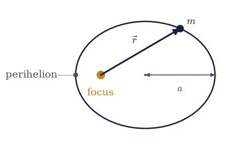
Fig. 89 Geometry of a bound Kepler orbit: the particle of mass \(m\) moves on an ellipse with the gravitating centre at one focus (amber), its position given by the radius vector \(\vec r\) from that focus; \(a\) is the semi-major axis and the perihelion marks the closest approach along the major axis.

---

Setup

Setup holds the units choice (\(GM = 1\), reduced mass \(\mu = 1\)), the bound initial condition S0_BOUND every orbit below is launched from, and one instrument: the event function the solver roots to stamp each perihelion passage. This notebook’s own physics is not here — you write the force law rhs in Exercise 1, the energy and the integration wrapper in Exercise 2, the angular momentum in Exercise 4, and the Laplace–Runge–Lenz vector in Exercise 8.

The Setup below holds this notebook’s data and instruments — nothing you are asked to build. It is collapsed so the building stays yours; expand it whenever you want the details.

Show code cell source

Hide code cell source

import numpy as np
from scipy.integrate import solve_ivp
import matplotlib.pyplot as plt

from ecp import draw, validate
from ecp.animate import show


GM = 1.0  # data: gravitational parameter (units choice); reduced mass mu = 1
# data: a bound elliptical initial condition — r = 1, purely tangential speed
# 1.2, which exceeds the circular speed 1.0, so this point is the perihelion.
S0_BOUND = np.array([1.0, 0.0, 0.0, 1.2])


# instrument: perihelion detection, not the lesson — this is the root the
# solver watches for so it can stamp each closest approach; the physics read
# off those stamps (the period in Exercise 6, the apsidal advance in
# Exercises 5 and 7) is what the exercises are about.
def perihelion_event(t, s, beta):
    """Event: zero when the radial velocity vanishes (selects minima of r)."""
    x, y, vx, vy = s
    return x * vx + y * vy  # = r * dr/dt


perihelion_event.direction = 1.0  # r increasing through zero -> perihelion

Exercise 1 — Implement the equation of motion

In the theory section we wrote the central-force law, Eq. 108: the acceleration points straight back toward the centre, anti-parallel to \(\hat{\mathbf r}\), with magnitude \(1/r^{\beta}\). Everything else in the notebook (the orbit, the conserved quantities, the period) follows from integrating this one vector equation. This exercise turns Eq. 108 into code and checks it at a test point before we trust it downstream.

1. Using Eq. 108, write rhs(t, s, beta=2.0) for the state \(\mathbf s = (x, y, v_x, v_y)\), returning \((\dot x, \dot y, \dot v_x, \dot v_y)\) (numpy.hypot for \(r\)). Write this one yourself — the implementation is the lesson.

2. Evaluate the acceleration at a test state and confirm it equals \(-\hat{\mathbf r}/r^{2}\) for the Newtonian case \(\beta = 2\) — the validation below does exactly this.

Validation 1 — the acceleration is \(-GM/r^2\,\hat{\mathbf r}\)

At a test position the acceleration returned by rhs (its last two components) must point anti-parallel to the radial unit vector with magnitude \(1/r^2\). If this ✗-es, look first at the sign and at the power of \(r\) in rhs.

✓  acceleration is -GM/r² r̂ (β=2)   [max|Δ| = 0 (rtol=1e-10, atol=1e-09)]

True

Exercise 2 — Integrate a bound orbit and plot it

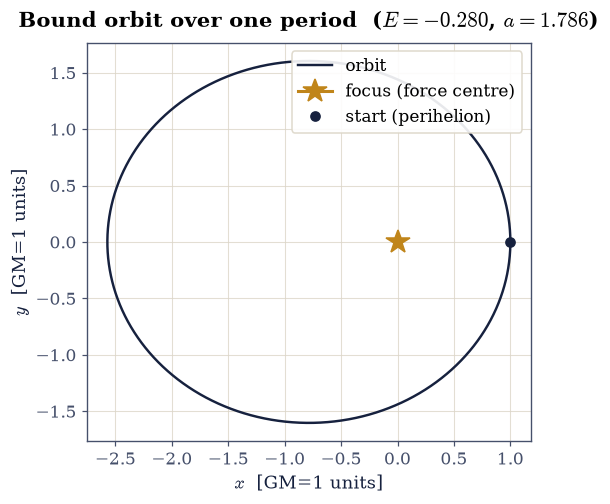
With Eq. 108 in hand, the orbit is fixed entirely by the initial position and velocity. We launch from S0_BOUND: radius 1 with a purely tangential speed of 1.2, faster than the circular speed 1.0, so the orbit is a bound ellipse with the force centre at one focus. How long “one period” is, though, is not known in advance: the energy Eq. 109 fixes the semi-major axis through vis-viva Eq. 111, and Kepler’s third law Eq. 112 turns that axis into a period. The orbit’s clock therefore comes from its energy, which is why the energy is written here — before Exercises 3 and 4 turn it and the angular momentum into integrator checks.

1. Using Eq. 109, write energy(s, beta=2.0), the specific energy \(E = \tfrac12 v^2 + r^{1-\beta}/(1-\beta)\), evaluating on a single state \((x, y, v_x, v_y)\) or on a whole state history alike. Write this one yourself — the implementation is the lesson.

2. Package the integration as integrate(s0, t_end, beta=2.0, n=4000): scipy.integrate.solve_ivp on Eq. 108 with the DOP853 high-order integrator, tight tolerances, and a dense uniform t_eval grid so the curve is smooth rather than a chain of straight segments.

3. Set the reference orbit’s clock: \(E_0\) from Part 1, then \(a = -1/(2E_0)\) and \(T = 2\pi\sqrt{a^3}\); integrate from S0_BOUND over exactly that one period.

4. Plot \(y\) vs \(x\) with equal aspect, mark the focus at the origin, and confirm by eye that the ellipse closes.

Exercise 3 — Energy as an integrator check

The energy Eq. 109 is conserved by the exact dynamics, so any drift in the computed energy along the trajectory is pure numerical error. This is the canonical “did I integrate it correctly?” test. This exercise evaluates Eq. 109 along the orbit from Exercise 2 and plots its relative drift.

1. With the energy you wrote in Exercise 2, compute \(E(t)\) along that exercise’s trajectory.

2. Plot the relative drift \((E - E_0)/|E_0|\) and confirm it stays at the level of the solver tolerance — the validation makes this quantitative.

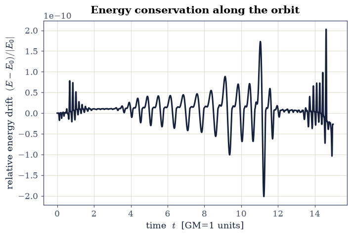
✓  total energy conserved (integrator check)   [max relative drift = 2.02703e-10 (limit 1e-06)]

True

Exercise 4 — Angular-momentum conservation

A central force exerts no torque about the centre, so the angular momentum Eq. 110 is the orbit’s second constant of motion, and the geometric content of Kepler’s second law: the radius vector sweeps equal areas in equal times, because the areal rate is exactly \(L_z/2\). In the plane the angular momentum has only its out-of-plane component, so the whole vector collapses to the single scalar \(L_z = x v_y - y v_x\).

1. Using Eq. 110, write Lz(s), evaluating on a single state \((x, y, v_x, v_y)\) or on a whole state history alike.

2. Compute \(L_z(t)\) along the trajectory of Exercise 2 and plot its relative drift.

3. As a visual of Kepler’s second law, shade the area swept over one short early interval and one short late interval and note they are equal for equal elapsed time.

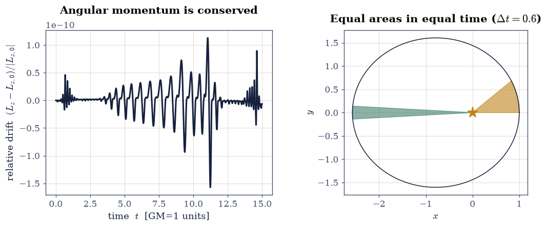
✓  angular momentum L_z conserved   [max relative drift = 1.57144e-10 (limit 1e-06)]

True

With your assistant

Ask your assistant for orbit-integration code for this potential, written any way it likes — then hold it to the two gates this notebook just built: energy flat to Exercise 3’s tolerance, angular momentum flat to Exercise 4’s. A physics-flavored check outranks any code review: whoever wrote the code, the conservation laws are not negotiable. The check is yours.

Exercise 5 — The inverse-square orbit closes (worked animation)

Bertrand’s theorem (theory section) promises that the inverse-square ellipse closes exactly: after one radial period the orbit returns to the same point moving the same way, so it retraces a single curve forever. This exercise makes that visible and then measures it.

This is the worked animation of the notebook: study how it is built. It animates the body tracing the ellipse with a trailing path over two periods; the trail lands exactly on top of itself, which is what “closed” means. The validation does not look at the animation at all: it measures the apsidal advance: the change in polar angle between successive perihelia, minus \(2\pi\). For a closed orbit that advance is zero.

Once Loop Reflect

Fig. 90 Animation of the inverse-square (\(\beta=2\)) bound orbit over two radial periods: the dark body traces the ellipse about the gravitating centre (amber star) while the amber trail retraces a single closed curve, the signature of zero apsidal advance demanded by Bertrand’s theorem.

Validation 5 — the orbit closes (zero apsidal advance)

We integrate several radial periods, locate each perihelion as a minimum of \(r\) (a zero of \(\dot r\) with \(r\) increasing), unwrap the polar angle, and measure the angle gained between consecutive perihelia. Subtracting \(2\pi\) gives the apsidal advance, which must be ≈ 0 for the inverse-square law. A ✗ here points at the perihelion detection or the angle unwrapping, not at any drawing code.

✓  inverse-square orbit closes (zero apsidal advance)   [got 1.13806e-08 vs expected 0 (rtol=1e-06, atol=0.1)]

True

Exercise 6 — Kepler’s third law

Kepler’s third law Eq. 112 says the period depends only on the semi-major axis: \(T = 2\pi\sqrt{a^3}\) in our units. We can get \(a\) without ever measuring the orbit’s geometry (the vis-viva relation Eq. 111 gives it straight from the energy), and we can measure \(T\) directly as the time between perihelion passages. This exercise compares the two.

1. With the energy you wrote in Exercise 2 and Eq. 111, compute the semi-major axis \(a = -1/(2E)\) of the reference orbit.

2. Measure the radial period as the mean perihelion-to-perihelion time (the perihelion_event located by solve_ivp) and compare it to Eq. 112.

3. Repeat for a few launch speeds and confirm \(T^2\) is linear in \(a^3\).

a = 1.785714   T_measured = 14.993321   2π√(a³) = 14.993321

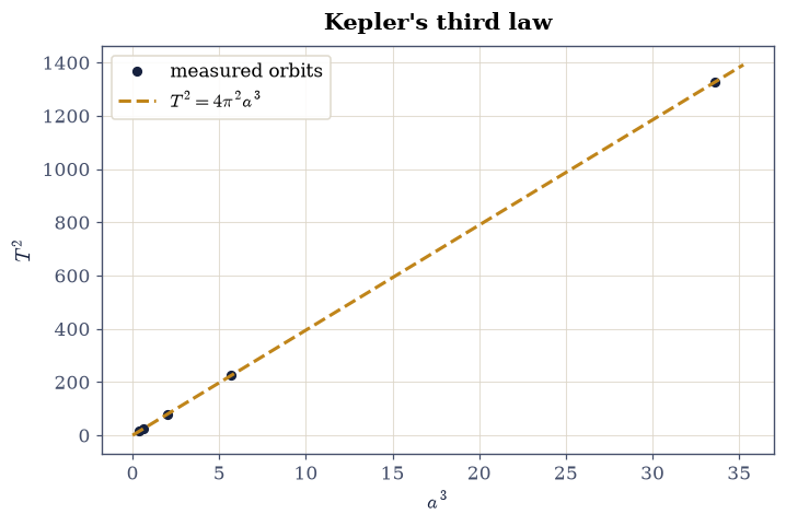
✓  period obeys Kepler's third law   [got 14.9933 vs expected 14.9933 (rtol=0.001, atol=1e-09)]

True

Exercise 7 — Precession under a modified force law (student animation)

Bertrand’s theorem cuts the other way too: change the exponent away from \(\beta = 2\) and the orbit cannot close: it precesses. We set \(\beta = 2.1\), a small change to Eq. 108, and the ellipse becomes a slowly rotating rosette. This is the student-implemented animation: the setup and the data are given; you write the player.

1. Integrate Eq. 108 with \(\beta = 2.1\) from S0_BOUND over several periods using scipy.integrate.solve_ivp (DOP853) on a dense t_eval, and store the trajectory (x, y).

2. Build a FuncAnimation of the body tracing the rosette with a trailing path — there are many valid ways to do this — then plt.close(fig) and end the cell with ecp.animate.show(anim).

The validation below checks the physics of the animated orbit, not the drawing code: it measures the apsidal advance and confirms it is clearly nonzero (the orbit precesses). A ✗ means “re-check the β=2.1 trajectory or the apsidal measurement,” never “the animation is wrong.”

Once Loop Reflect

Fig. 91 Animation of the orbit under the modified force-law exponent \(\beta=2.1\) over six radial periods: the amber body traces a slowly rotating rosette (dark trail) about the force centre (amber star), the open, precessing orbit Bertrand’s theorem predicts for any \(\beta\neq2\).

Validation 7 — the modified force law precesses

Same apsidal-advance measurement as Exercise 5, now for \(\beta = 2.1\). We expect a clearly nonzero advance per radial period (it comes out near \(+21^\circ\)), the quantitative signature of a non-closing orbit.

apsidal advance per radial period ≈ 20.92°
✓  modified force law makes the orbit precess   [apsidal advance = 20.92° per radial period]

True

Exercise 8 — The orbit that closes: the Laplace–Runge–Lenz vector

Exercise 5 showed the inverse-square orbit retraces a single closed ellipse, and Exercise 7 showed that the smallest change to the force law sets it precessing. What conserved quantity marks the difference? For the \(1/r^2\) force, and only for it, there is an extra conserved vector beyond energy and angular momentum: the Laplace–Runge–Lenz vector

\[\mathbf A=\mathbf v\times\mathbf L-k\,\hat{\mathbf r},\]

which points along the major axis toward perihelion. Its constancy is the closure of the orbit: a fixed \(\mathbf A\) means the perihelion never moves. This is the clean instrument for the whole question — it reads the closure off directly from the conserved vector, with no need to hunt for minima of \(r\) — and it is the deepest fact about the Kepler problem. The smallest departure from \(1/r^2\) destroys this conservation, and the orbit begins to turn.

In the plane the angular momentum has only its out-of-plane component \(L_z\) Eq. 110, so the cross product collapses to two components, \(\mathbf A=(L_z v_y - k x/r,\; -L_z v_x - k y/r)\). The length has a closed form too: \(|\mathbf A|/k = e = \sqrt{1 + 2EL_z^2/k^2}\), the orbit’s eccentricity written in the two constants of motion we already have. Everything below uses the same reference orbit (S0_BOUND, \(GM = 1\)).

1. Write lrl_vector(s, k=GM), returning \((A_x, A_y)\) for a single state or a whole state history alike. Write this one yourself — the implementation is the lesson.

2. Evaluate it along a trajectory integrated over thirty radial periods, with the integrate you wrote in Exercise 2.

3. Confirm its direction is fixed to within numerical noise (numpy.arctan2 of its components) — the orbit is exactly closed, no precession.

4. Confirm its length is \(|\mathbf A|/k=e\), against the closed form above evaluated with the energy of Exercise 2 and the Lz of Exercise 4.

reference orbit: e = 0.4400
LRL direction wanders by 1.01e-07° = 0.0004″ over 30 orbits
|A|/k = 0.4400  vs  eccentricity e = 0.4400

Validation 8 — the LRL vector is conserved (the orbit is exactly closed)

✓  the Laplace–Runge–Lenz vector is conserved — the Kepler orbit is exactly closed, with no precession   [got 1.01147e-07 vs expected 0 (rtol=1e-06, atol=0.001)]
✓  the LRL vector's length encodes the eccentricity, |A|/k = e   [got 0.44 vs expected 0.44 (rtol=0.001, atol=1e-09)]

True

Fig. 92 The closed Kepler ellipse with its conserved Laplace–Runge–Lenz vector \(\mathbf A\) (amber arrow) pointing from the force centre (star) along the major axis toward perihelion. Because \(\mathbf A\) is constant for the \(1/r^2\) force — its direction wandering by less than a thousandth of a degree over thirty orbits — the perihelion never moves and the ellipse retraces itself exactly. This perfect closure is special to the inverse-square law; the next two volumes show what happens when it breaks.

A thread to follow. This perfect closure is not generic; it is a property of the inverse-square force (among the falloff laws). Real planetary orbits precess slightly, and we now have, in our own code, everything needed to see why. §2.4 shows that the smallest departure from \(1/r^2\) sets the perihelion turning, at a rate we can predict and measure; and the general-relativity capstone (§4.8) shows that Mercury’s leftover precession — the part no Newtonian gravity explains — is one of relativity’s first triumphs. The puzzle is one the reader uncovers; relativity supplies the missing piece.

Notebook summary

• The inverse-square two-body problem (\(\ddot{\mathbf r}=-GM\hat{\mathbf r}/r^2\)) integrated to a closed bound orbit, with total energy and the angular momentum \(L_z\) conserved as integrator checks.

• Kepler’s third law \(T^2\propto a^3\) recovered across orbits, the closure of the inverse-square ellipse, and the precession that appears once the force law is modified away from \(1/r^2\).

• The Laplace–Runge–Lenz vector \(\mathbf A=\mathbf v\times\mathbf L-k\,\hat{\mathbf r}\) conserved for the \(1/r^2\) force (direction fixed to \(<10^{-3}\,\)° over thirty orbits, length \(|\mathbf A|/k=e\)): the exact statement that the orbit closes, and the opening of a thread — the orbit closes here, precesses in §2.4, and yields Mercury’s relativistic \(43''\)/century in §4.8.

Outlook

• Map the apsidal advance as a function of \(\beta\) across, say, \(1.8\)–\(2.2\) and watch it pass through zero exactly at the inverse-square law: a numerical reading of Bertrand’s theorem.

• Add a small relativistic \(1/r^3\) correction to the force and tune it to reproduce a Mercury-like perihelion precession.

• Push the launch speed past escape (\(v_0 > \sqrt{2}\) at \(r=1\)): the orbit becomes an unbound hyperbolic flyby. Measure the deflection angle versus impact parameter: the bridge to central-force scattering in Volume II.

References

[GPS02] (1,2,3)

Herbert Goldstein, Charles P. Poole, and John L. Safko. Classical Mechanics. Pearson, 3 edition, 2002.

[Nol16]

Wolfgang Nolting. Theoretical Physics 1: Classical Mechanics. Springer, 2016. Grundkurs Theoretische Physik 1.

Take this notebook with you

Use the download button (↓) in the toolbar above to save this notebook and run it yourself. The published notebooks ship without worked solutions; if you would like the reference solutions — to teach from or to check your own work — get in touch: hello@ramador.me.