


3.15 Waves in Media: Dispersion, Absorption, and the Fresnel Relations#
Notebook overview#
§3.8 built a wave and set it loose in empty space, where it travels at \(c\) and never changes. §3.13 put fields into matter but held them still. This notebook is where the two meet, and it is the one both of them promised: a wave arriving in a material, and the material answering back.
The whole of it comes out of a single mechanical picture. An electron bound in an atom is a mass on a spring with friction, so a passing light wave drives it exactly as the torque drove the pendulum in §1.2. That is not an analogy offered for comfort: it is the same differential equation, and we integrate it here with the same solver to check it against the same resonance curve. Multiply one electron’s response by the number density and the material’s permittivity becomes a function of frequency, \(\varepsilon(\omega)\), complex because the electron lags the drive. From there everything follows by algebra we can compute rather than quote. The square root of \(\varepsilon\) is a complex refractive index \(\tilde n = n + i\kappa\) whose real part slows the wave and whose imaginary part eats it; near the resonance \(n\) decreases with frequency, the anomalous dispersion that makes a prism misbehave where it also absorbs. Set the spring constant to zero and the bound electron becomes a free one: the Drude conductor, whose absorption length is the skin depth (9.2 mm in copper at 50 Hz, 65 µm at 1 MHz), and whose \(\varepsilon\) crosses zero at the plasma frequency. Below that frequency a free-electron gas reflects everything, which is why aluminium is a mirror up to 15.8 eV and why a 1 MHz radio signal bounces off the ionosphere while a 100 MHz one is lost to space.
The second half is the interface. A boundary condition has to hold at every point of the surface at once, and that single requirement forces the three waves to share a tangential wavevector: Snell’s law is phase matching, and we show it by measuring the mismatch as a function of the assumed refraction angle and watching it collapse to zero at Snell’s angle and nowhere else. The amplitudes then come from the jump conditions of §3.13, which for each polarization are two linear equations in two unknowns: we assemble that \(2\times2\) system and solve it, and out come the Fresnel relations. They pay immediate dividends. For one polarization the reflected amplitude passes through zero at Brewster’s angle, \(56.31^\circ\) for glass, because there the radiating dipoles in the medium point straight along the reflected ray and a dipole cannot radiate along its own axis (§3.10). Beyond the critical angle the refraction angle stops being real, the reflection becomes total, and the field that persists on the far side is evanescent: it travels along the surface, decays over 285 nm, is larger in amplitude than the incident wave, and carries exactly zero energy away. That last figure is the notebook’s one animation, because it is the one place where something genuinely moves.
Everything is in SI units, with the CODATA constants imported from
scipy.constants. The material model is a single Lorentz resonance in the ultraviolet
(\(\hbar\omega_0 = 10\) eV, \(\hbar\gamma = 0.5\) eV, bound-electron density
\(n_b = 9.07\times10^{28}\,\mathrm{m^{-3}}\)), chosen so that its static limit is
\(\varepsilon_r(0) = 2.25\), i.e. \(n = 1.50\): the index of ordinary glass, out of one
resonance. Every optics exercise from Exercise 6 onward uses that same \(n = 1.5\), so
the second half of the notebook is running on the number the first half computed.
How to read the checks. Each exercise ends with a
validatecall against an independent fact: an integrated trajectory against a closed-form complex amplitude, \(n^2-\kappa^2=\operatorname{Re}\varepsilon_r\), copper’s conductivity against its measured \(5.96\times10^7\,\)S/m, aluminium’s plasma energy against the measured 15.8 eV, \(R+T=1\) at every angle of incidence, \(|r|=1\) beyond the critical angle. A validation compares a result to an expected physical fact, so a ✗ does not by itself mean the answer is wrong: it may be a genuine error, a different-but-valid convention (a sign, a branch of a square root), or too tight a tolerance. Treat a ✗ as a prompt to locate the discrepancy. Passing is strong evidence, not proof.A sign-convention note. We write plane waves as \(e^{i(\tilde k z-\omega t)}\) throughout. With that choice a passive medium has \(\operatorname{Im}\varepsilon_r>0\) and \(\operatorname{Im}\tilde n\ge0\), which is the branch
numpy.sqrtreturns for a complex argument. The opposite convention \(e^{i(\omega t-\tilde k z)}\), common in engineering, flips the sign of every imaginary part; a check that fails only in the sign of \(\kappa\) has found the convention, not an error.
Theory in brief#
The Lorentz oscillator#
Bind an electron of charge \(-e\) and mass \(m\) to its atom with a restoring force \(-m\omega_0^2 x\), let it lose energy at rate \(\gamma\), and drive it with the electric field of a passing wave, \(E(t)=E_0\cos\omega t\). Newton’s second law reads
which is the damped, driven harmonic oscillator of §1.2 with light supplying the drive. Writing \(x(t)=\operatorname{Re}\bigl[\tilde x\,E_0 e^{-i\omega t}\bigr]\), the steady state is fixed by one complex number,
whose modulus is the resonance curve and whose argument fixes the phase by which the electron lags the force driving it. Since that force is \(-eE\), the lag is \(\pi+\arg\tilde x\), and it runs from \(0\) well below resonance through exactly \(\pi/2\) at \(\omega=\omega_0\) to \(\pi\) well above: the electron follows the push at low frequency and opposes it at high frequency, which is why \(\varepsilon_r\) changes sign.
The dielectric function#
Each displaced electron carries a dipole moment \(-e\,x\), so a density \(n_b\) of them gives a polarization \(P=-e\,n_b x = \varepsilon_0\chi_e E\). Feeding Eq. 276 into \(\varepsilon_r = 1+\chi_e\) gives the dielectric function
the frequency-dependent, complex successor to the constant \(\varepsilon_r\) of §3.13. It is complex because the electron lags, and a lagging response means work done on the medium: absorption. Its static value \(\varepsilon_r(0)=1+\omega_p^2/\omega_0^2\) is the ordinary permittivity, and it returns to \(1\) far above resonance, where the electron is too heavy to keep up and the material might as well be vacuum. Between \(\omega_0\) and \(\omega_L=\sqrt{\omega_0^2+\omega_p^2}\) a strong resonance drives \(\operatorname{Re}\varepsilon_r\) negative, a band in which no wave propagates.
The complex refractive index#
Maxwell’s equations in a medium are those of §3.8 with \(\varepsilon_0\to\varepsilon_0\varepsilon_r\), so a plane wave \(e^{i(\tilde kz-\omega t)}\) has \(\tilde k=\tilde n\,\omega/c\) with
The split is the whole story of optics in one line. The real part \(n\) slows the phase to \(c/n\) and bends rays; the imaginary part \(\kappa\) (the extinction coefficient) multiplies the field by \(e^{-\omega\kappa z/c}\), so the intensity obeys Beer’s law
Away from resonance \(n\) rises with frequency (blue bends more than red: normal dispersion). Inside the absorption line it falls — anomalous dispersion — and the two facts are not independent: absorption and dispersion are the imaginary and real parts of one analytic function, which is the content of the Kramers–Kronig relations derived in §7.2. We use nothing from there here; this notebook computes both parts directly from Eq. 277 and simply observes that they peak together.
Free electrons: Drude, skin depth, plasma frequency#
Take away the spring. With \(\omega_0=0\) and \(\gamma=1/\tau\) the collision rate, Eq. 277 becomes the Drude dielectric function of a conductor,
so the conduction current of Ohm’s law is what a polarization current becomes when nothing holds the charge back. At low frequency the second form dominates, \(\tilde n\simeq(1+i)\sqrt{\sigma/2\varepsilon_0\omega}\), and the field falls off inside the metal over the skin depth
a millimetre-scale length at mains frequency and a micron at a gigahertz: high-frequency current rides on the surface of a wire. At the other end, when \(\omega\tau\gg1\) collisions are irrelevant and Eq. 280 collapses to
negative below the plasma frequency \(\omega_p\) and positive above it. Negative \(\varepsilon_r\) means purely imaginary \(\tilde n\): the wave cannot propagate, it decays, and with no absorption to accompany the decay it is reflected in full. That single sign change explains the shine of a clean metal, the ultraviolet transparency window of aluminium, and the fact that the ionosphere is a mirror for the AM band and a window for FM.
Snell’s law is phase matching#
At a flat interface the boundary conditions of §3.13 — \(E_\parallel\) and \(H_\parallel\) continuous — must hold at every point of the surface, at every instant. The three waves therefore have to agree in their variation along the surface, which forces one frequency and one tangential wavevector on all of them. With \(k_j=n_j\omega/c\) that is
the law of reflection and Snell’s law, obtained without ever writing an amplitude.
The Fresnel relations#
The amplitudes come next, from the same two continuity conditions, and they depend on polarization. For s-polarization (\(\mathbf E\) perpendicular to the plane of incidence) continuity of \(E_\parallel\) and of \(H_\parallel\) reads \(1+r_s=t_s\) and \(n_1\cos\theta_i(1-r_s)=n_2\cos\theta_t\,t_s\), whose solution is
For p-polarization (\(\mathbf E\) in the plane of incidence) the same two conditions read \(n_1(1+r_p)=n_2t_p\) and \(\cos\theta_i(1-r_p)=\cos\theta_t\,t_p\), giving
The measured quantities are the reflectance \(R=|r|^2\) and the transmittance \(T=(n_2\cos\theta_t/n_1\cos\theta_i)|t|^2\), whose geometric prefactor accounts for the beam’s change of cross-section and of speed; energy conservation is the statement \(R+T=1\).
Brewster’s angle, total internal reflection, the evanescent wave#
The numerator of \(r_p\) vanishes when \(n_2\cos\theta_i=n_1\cos\theta_t\), which with Eq. 283 happens at Brewster’s angle
The second form is the physical one: at \(\theta_B\) the dipoles driven in the second medium oscillate along the direction the reflected ray would take, and a dipole radiates nothing along its own axis (§3.10). Reflected light at \(\theta_B\) is purely s-polarized, which is what polarizing sunglasses exploit.
Going the other way, from glass into air, Eq. 283 has no real solution once \(\sin\theta_i>n_2/n_1\). Past that critical angle \(\theta_c=\arcsin(n_2/n_1)\) we set \(\cos\theta_t=i\,q\) with \(q=\sqrt{(n_1\sin\theta_i/n_2)^2-1}\), and the transmitted wave becomes evanescent,
travelling along the surface and dying within a fraction of a wavelength of it. Both Fresnel coefficients then have modulus one — the reflection is total — while \(|t|\) can exceed one, because the evanescent field stores energy near the surface without carrying any away. Frustrate that decay with a second piece of glass a few hundred nanometres off and the light crosses the gap: the optical analogue of quantum tunnelling, and the working principle of every fingerprint sensor and near-field microscope.
Setup#
Data and instruments only: the CODATA constants, the parameters of the model dielectric and of the three real materials the notebook grades itself against (copper, aluminium, the night-time ionosphere), the optical bench of a helium–neon wavelength and the two indices \(n=1\) and \(n=1.5\), the series palette, and one unit conversion between photon energy in electronvolts and angular frequency in rad/s. Nothing in the notebook’s own line of argument is pre-built: the equation of motion, the dielectric function, the complex index, the Drude limit, the phase-matching mismatch and the \(2\times2\) boundary-condition system that yields the Fresnel coefficients are all assembled in the exercises. Nothing here is stochastic.
The Setup below holds this notebook’s data and instruments — nothing you are asked to build. It is collapsed so the building stays yours; expand it whenever you want the details.
Exercise 1 — The Lorentz oscillator: the driven oscillator inside an atom (worked)#
An electron bound in an atom is a mass on a spring. Pull it a distance \(x\) off centre and the rest of the atom pulls back with \(-m\omega_0^2x\); let it radiate and collide and it loses energy at a rate \(\gamma\); send a light wave past and its electric field pushes on the charge \(-e\). Newton’s second law is then Eq. 275, and that equation is not merely like the damped driven pendulum of §1.2 in the small-angle regime: it is the same equation, with \(\ell\) and \(g\) replaced by an atom and light replacing the shaker. Everything that notebook found — a resonance peak, a phase lag growing from \(0\) through \(-\pi/2\) to \(-\pi\), a width set by the damping — is about to become the optics of glass (Fig. 300).
The steady state is one complex number, Eq. 276. Its modulus gives the amplitude and its argument the lag, and both are cleanly measurable from an integrated trajectory: writing the late-time motion as \(x(t)=\operatorname{Re}[X e^{-i\omega t}]\) means \(x(t)=\operatorname{Re}X\,\cos\omega t+\operatorname{Im}X\,\sin\omega t\), so projecting the sampled \(x(t)\) onto \(\cos\omega t\) and \(\sin\omega t\) over a whole number of drive periods returns \(X\) itself.
The oscillator here is the model dielectric’s: \(\hbar\omega_0=10\,\)eV, \(\hbar\gamma=0.5\,\)eV, driven by \(E_0=10^{5}\,\)V/m (an ordinary laboratory field, well inside the linear regime).
Part a) Write lorentz_rhs(t, s, omega_d) for the state \(s=(x,\dot x)\), returning
\((\dot x,\;-\omega_0^2x-\gamma\dot x-(e/m)E_0\cos\omega_d t)\) from Eq. 275, with
\(e\) and \(m\) the CODATA QE and ME. Write this one yourself — the implementation
is the lesson.
Part b) Integrate it from rest, \(x(0)=\dot x(0)=0\), at the drive frequency
\(\omega_d=0.8\,\omega_0\) for 60 drive periods with
scipy.integrate.solve_ivp(method="DOP853", rtol=1e-10, atol=1e-30) — a high-order
explicit Runge–Kutta at tight tolerance, because the quantity of interest is a phase
accumulated over sixty cycles — sampling the last ten periods on a
t_eval grid of 20001 points so the transient is gone and the projections of Part c
have a dense, whole-period window.
Part c) Extract the measured complex amplitude by the two projections
\(\operatorname{Re}X=(2/T_{\rm win})\int x\cos\omega_d t\,dt\) and
\(\operatorname{Im}X=(2/T_{\rm win})\int x\sin\omega_d t\,dt\), each evaluated with
numpy.trapezoid over the ten-period window \(T_{\rm win}\), and compare \(X\) with
\(\tilde x(\omega_d)E_0\) from Eq. 276.
Part d) Repeat the integration at 15 drive frequencies spaced linearly over \(\omega_d/\omega_0\in[0.2,\,1.8]\) and plot the measured amplitude \(|X|\) and the lag behind the driving force, \(\pi+\arg X\), against the closed-form curves \(|\tilde x(\omega)|E_0\) and \(\pi+\arg\tilde x(\omega)\) (Fig. 301). The lag passes through exactly \(\pi/2\) at \(\omega_d=\omega_0\), where the denominator of Eq. 276 is purely imaginary.
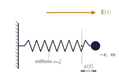
Fig. 300 The Lorentz oscillator: an electron of charge \(-e\) and mass \(m\) held to its atom by a spring of stiffness \(m\omega_0^2\) (so its free oscillation frequency is \(\omega_0\)), displaced by \(x(t)\) from its equilibrium position (dotted line, marked point) and driven along \(\hat{\mathbf x}\) by the electric field \(\mathbf E(t)=E_0\cos\omega t\,\hat{\mathbf x}\) of a passing light wave (amber). Energy loss to radiation and collisions enters as a damping rate \(\gamma\). This is the damped driven oscillator of the mechanics volume with light as the drive, and its steady-state complex amplitude is the refractive index of the material.#
drive at ω_d = 0.8 ω₀ (ħω_d = 8.0 eV)
measured X = -2.090847e-16-2.323091e-17j m
eq-wm-xamp = -2.090844e-16-2.323160e-17j m
|X| measured / closed form = 1.000001141
phase lag at ω_d = ω₀: 1.570796327 rad (π/2 = 1.570796327)
peak measured amplitude over the sweep = 1.524e-15 m
Validation 1#
✓ the integrated steady-state amplitude at ω_d = 0.8ω₀ matches eq-wm-xamp [got 2.10371e-16 vs expected 2.10371e-16 (rtol=0.001, atol=1e-09)]
✓ so does its phase arg X, which fixes how far the electron trails the field [got -3.03094 vs expected -3.03094 (rtol=0.001, atol=1e-09)]
✓ the swept resonance curve reproduces |x̃(ω)|E₀ across 0.2 ω₀ to 1.8 ω₀ [max|Δ| = 2.96377e-19 (rtol=0.01, atol=1e-09)]
✓ the lag behind the driving force is exactly π/2 on resonance [got 1.5708 vs expected 1.5708 (rtol=1e-09, atol=1e-09)]
True
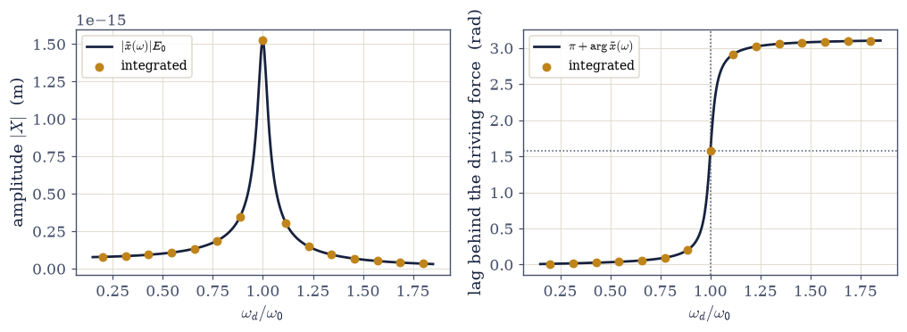
Fig. 301 The Lorentz oscillator’s steady-state response, integrated and compared with the closed form. Left: the displacement amplitude \(|X|\) measured from fifteen separate solve_ivp trajectories (amber points), each projected onto \(\cos\omega_d t\) and \(\sin\omega_d t\) over ten drive periods after fifty periods of settling, lying on \(|\tilde x(\omega)|E_0\) from eq-wm-xamp (dark curve). Right: the phase \(\pi+\arg X\) by which the electron lags the force driving it, rising from \(0\) far below resonance (it follows the push) through exactly \(\pi/2\) at \(\omega_d=\omega_0\) (dotted lines) toward \(\pi\) above it (it opposes the push). This is the resonance curve of the damped driven oscillator met in the mechanics volume, and the lag on the right is the reason the refractive index is complex.#
Exercise 2 — From one electron to \(\varepsilon(\omega)\) (student)#
One oscillator is a curiosity; a cubic metre of them is a material. An electron displaced by \(x\) carries a dipole moment \(-ex\), so a density \(n_b\) of identical bound electrons gives a polarization \(P=-e\,n_b\,x\), and with the steady state Eq. 276 that polarization is proportional to the field it responds to. Reading off the susceptibility from \(P=\varepsilon_0\chi_e E\) and adding the vacuum term gives the dielectric function Eq. 277, with the combination \(\omega_p^2=n_be^2/\varepsilon_0m\) collecting the density, charge and mass into a single frequency. The constant \(\varepsilon_r\) that §3.13 worked with is now a curve, and a complex one.
Three of its features are worth locating rather than admiring. Its static value \(\varepsilon_r(0)=1+\omega_p^2/\omega_0^2\) is the permittivity a capacitor would measure. Far above resonance the binding stops mattering at all, since \(\omega^2\gg\omega_0^2\) makes the denominator of Eq. 277 into \(-\omega^2\) and leaves \(\varepsilon_r\to1-\omega_p^2/\omega^2\): a free-electron response, which is exactly the plasma dielectric function Eq. 282 that Exercise 5 is about. The approach to the vacuum value \(1\) is therefore slow, from below. In between, if the resonance is strong enough, \(\operatorname{Re}\varepsilon_r\) dips below zero over a band, ending at the zero \(\omega_L=\sqrt{\omega_0^2+\omega_p^2}\) — a band where the wave cannot propagate at all, and the same zero that will reappear in Exercise 5 as the plasma frequency once \(\omega_0\) is set to zero.
The material is the model dielectric of Exercise 1: \(\hbar\omega_0=10\,\)eV, \(\hbar\gamma=0.5\,\)eV, \(n_b=9.07\times10^{28}\,\mathrm{m^{-3}}\).
Part a) Build \(\omega_p^2=n_be^2/(\varepsilon_0 m)\) from the Setup constants, then
evaluate Eq. 277 as an explicit complex numpy array on 4001 photon
energies spaced linearly over \(\hbar\omega\in[0.05,\,30]\,\)eV (converted to rad/s with
omega_from_eV), and plot \(\operatorname{Re}\varepsilon_r\) and
\(\operatorname{Im}\varepsilon_r\) (Fig. 302).
Part b) Report \(\varepsilon_r\) at the lowest grid energy against the static value \(1+\omega_p^2/\omega_0^2\), and at \(30\,\)eV against the free-electron form \(1-\omega_p^2/\omega^2\).
Part c) Locate the zero of \(\operatorname{Re}\varepsilon_r\) above the resonance with
scipy.optimize.brentq bracketed on \([11,\,20]\,\)eV, and compare it with
\(\hbar\omega_L=\hbar\sqrt{\omega_0^2+\omega_p^2}\). The small offset between them is the
damping’s doing, and it shrinks with \(\gamma\).
Part d) Report the energy band on which \(\operatorname{Re}\varepsilon_r<0\) (a
numpy boolean mask over the grid), and confirm with numpy.all that
\(\operatorname{Im}\varepsilon_r>0\) everywhere on the grid — a passive medium absorbs
energy at every frequency and supplies it at none.
ħω_p = 11.183 eV
ε_r(0.05 eV) = 2.250641+0.000313j vs 1 + ω_p²/ω₀² = 2.250610
ε_r(30 eV) = 0.843729+0.002930j vs 1 − ω_p²/ω² = 0.861043
Re ε_r = 0 at ħω = 14.9870 eV vs ħω_L = 15.0020 eV
Re ε_r < 0 on ħω ∈ [10.02, 14.98] eV — no propagation there
Im ε_r > 0 at every grid frequency (a passive medium): True
Validation 2#
✓ the static limit of ε_r(ω) is 1 + ω_p²/ω₀² = 2.2506, the permittivity of §3.13 [got 2.25064 vs expected 2.25061 (rtol=0.0001, atol=1e-09)]
✓ far above resonance the binding is irrelevant and ε_r → 1 − ω_p²/ω², the free-electron form of Exercise 5 [got 0.843729 vs expected 0.861043 (rtol=0.03, atol=1e-09)]
✓ Re ε_r crosses zero at ω_L = √(ω₀² + ω_p²), the top of the no-propagation band [got 2.27693e+16 vs expected 2.27921e+16 (rtol=0.005, atol=1e-09)]
✓ Im ε_r > 0 at every frequency: the medium absorbs energy and never supplies it
True
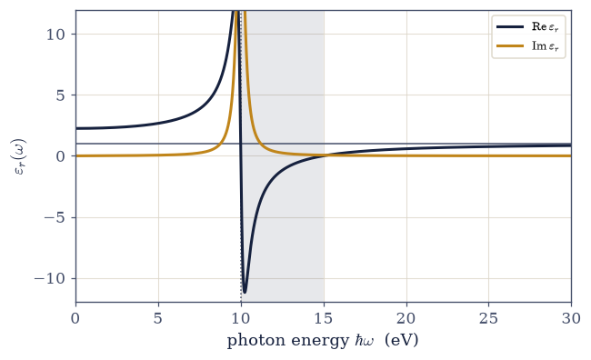
Fig. 302 The dielectric function of the model material, one Lorentz resonance at \(\hbar\omega_0=10\) eV with \(\hbar\gamma=0.5\) eV. The real part (dark) starts at the static permittivity \(2.2506\), swings up and then steeply down through the resonance (dotted vertical), and crosses zero at \(\hbar\omega_L=\hbar\sqrt{\omega_0^2+\omega_p^2}=15.0\) eV before climbing slowly back toward the vacuum value \(1\) (grey line) along the free-electron curve \(1-\omega_p^2/\omega^2\), still only \(0.84\) at 30 eV. The imaginary part (amber) is a peak centred on the resonance and positive everywhere: it is the absorption, and its positivity is the statement that the medium takes energy from the wave at every frequency. The shaded band is where \(\operatorname{Re}\varepsilon_r<0\) and no wave propagates at all.#
Exercise 3 — The complex refractive index, and anomalous dispersion (student)#
Maxwell’s equations inside a linear medium are those of §3.8 with \(\varepsilon_0\) replaced by \(\varepsilon_0\varepsilon_r(\omega)\), so a plane wave \(e^{i(\tilde kz-\omega t)}\) travels with \(\tilde k=\tilde n\,\omega/c\) and a complex refractive index \(\tilde n=\sqrt{\varepsilon_r}\), Eq. 278. Splitting it as \(\tilde n=n+i\kappa\) splits the physics with it: the factor \(e^{i\omega nz/c}\) is a wave whose phase velocity is \(c/n\), and the factor \(e^{-\omega\kappa z/c}\) is a decay. Intensity goes as the modulus squared, hence Beer’s law Eq. 279 with absorption coefficient \(\alpha=2\omega\kappa/c\). One square root of one complex function has produced both of the things a material does to light.
Squaring \(\tilde n=n+i\kappa\) ties the two halves to the two halves of \(\varepsilon_r\): \(n^2-\kappa^2=\operatorname{Re}\varepsilon_r\) and \(2n\kappa=\operatorname{Im}\varepsilon_r\). Those identities are the sharp test that the right branch of the square root has been taken, since \(\sqrt{\varepsilon_r}\) has two values and only the one with \(\kappa\ge0\) describes a wave that decays as it goes.
The behaviour worth hunting for is anomalous dispersion. Outside an absorption line \(n\) increases with frequency, which is why a prism bends blue more than red; inside the line \(n\) falls, so briefly the prism runs backwards. The two effects are not independent, because \(\operatorname{Re}\varepsilon_r\) and \(\operatorname{Im}\varepsilon_r\) are the real and imaginary parts of one analytic function — the Kramers–Kronig statement proved in §7.2. Nothing here depends on that result; we simply compute both parts from Eq. 277 and find them peaked together.
The material is again the model dielectric (\(\hbar\omega_0=10\,\)eV, \(\hbar\gamma=0.5\,\)eV, \(n_b=9.07\times10^{28}\,\mathrm{m^{-3}}\)), on the same \(\hbar\omega\in[0.05,\,30]\,\)eV grid of 4001 points built in Exercise 2.
Part a) Form \(\tilde n=\) numpy.sqrt of the complex array eps_model of Exercise 2
(numpy returns the principal branch, the one with \(\operatorname{Im}\tilde n\ge0\)), take
.real and .imag for \(n\) and \(\kappa\), and plot both (Fig. 303).
Part b) Confirm the branch with numpy.allclose on the two identities of
Eq. 278, \(n^2-\kappa^2=\operatorname{Re}\varepsilon_r\) and
\(2n\kappa=\operatorname{Im}\varepsilon_r\), and report \(n\) and \(\kappa\) at the lowest grid
energy: \(n\to\sqrt{2.2506}=1.500\), the glass index the rest of the notebook uses, and
\(\kappa\to0\).
Part c) Compute \(\alpha=2\omega\kappa/c\) from Eq. 279 and report the absorption length \(1/\alpha\) at \(\hbar\omega=2\,\)eV (visible light, far below the line) and at \(\hbar\omega=\hbar\omega_0=10\,\)eV (dead centre).
Part d) Differentiate \(n(\omega)\) with numpy.gradient on the \(\omega\) grid and mask
where \(dn/d\omega<0\): that band is the anomalous dispersion. Confirm it is one contiguous
interval (numpy.diff of the masked indices is all ones), that the absorption peak
\(\arg\max\operatorname{Im}\varepsilon_r\) lies inside it, and that \(dn/d\omega>0\) at both
\(2\,\)eV and \(25\,\)eV, where dispersion is normal.
n² − κ² = Re ε_r : True; 2nκ = Im ε_r : True
at 0.05 eV: n = 1.500214 (√2.2506 = 1.500203), κ = 1.042e-04
1/α at 2 eV = 11.07 µm (n = 1.5174)
1/α at 10 eV = 2.84 nm (n = 3.6012)
anomalous band: ħω ∈ [9.85, 13.77] eV, contiguous: True
absorption peak at 9.99 eV lies inside it: True
dispersion normal at 2 eV and 25 eV: True
Validation 3#
✓ the square root took the physical branch: n² − κ² = Re ε_r and 2nκ = Im ε_r
✓ the static index is √ε_r(0) = 1.500 — the glass value used from Exercise 6 on [got 1.50021 vs expected 1.5002 (rtol=0.0001, atol=1e-09)]
✓ and κ → 0 there: far below resonance the medium is transparent [got 0.000104208 vs expected 0 (rtol=1e-06, atol=0.001)]
✓ anomalous dispersion (dn/dω < 0) occupies one band that contains the absorption peak, with normal dispersion on both sides of it
True
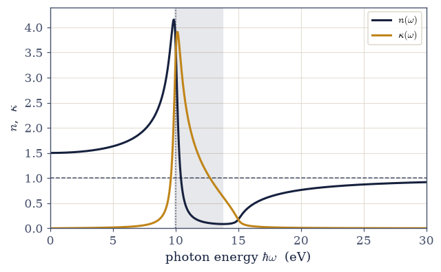
Fig. 303 The complex refractive index \(\tilde n=n+i\kappa=\sqrt{\varepsilon_r}\) of the model dielectric. The real part (dark) begins at \(1.500\), the index of glass, and climbs with frequency — normal dispersion, blue bent more than red — until the resonance at \(\hbar\omega_0=10\) eV (dotted vertical), where it turns over and falls steeply. The extinction coefficient \(\kappa\) (amber) is the absorption, peaked on the line. The shaded band is where \(dn/d\omega<0\): anomalous dispersion, which occurs only where the medium also absorbs, and which contains the absorption peak. The dashed line marks the vacuum value \(n=1\), which the real index drops below above the resonance (a phase velocity greater than \(c\), and no signal faster than \(c\): the group velocity is what carries information).#
Exercise 4 — Free electrons, absorption, and the skin depth (student)#
Now take the spring away. In a metal the conduction electrons are bound to no particular atom, so \(\omega_0=0\) and the only thing opposing the drive is the scattering that gives a relaxation time \(\tau\), i.e. \(\gamma=1/\tau\). Putting those into Eq. 277 gives the Drude dielectric function Eq. 280. Expanding it for \(\omega\tau\ll1\) leaves \(\varepsilon_r\simeq i\sigma/\varepsilon_0\omega\) with \(\sigma=ne^2\tau/m\), which is worth pausing on: Ohm’s law is not a separate piece of physics bolted onto the theory, it is what the polarization response of Exercise 2 becomes when nothing holds the charge in place (Fig. 304).
A purely imaginary \(\varepsilon_r\) has \(\tilde n=(1+i)\sqrt{\sigma/2\varepsilon_0\omega}\), equal real and imaginary parts, so a metal at low frequency attenuates a wave over the same distance in which it turns it through a radian. That distance is the skin depth Eq. 281, \(\delta=c/\omega\kappa\simeq\sqrt{2/\mu_0\sigma\omega}\), and it is the reason a mains busbar is solid while a radio-frequency conductor is a thin plated tube: above a few megahertz the current rides in a skin microns thick and the interior of the metal is dead weight.
The metal here is copper, with \(n=8.47\times10^{28}\,\mathrm{m^{-3}}\) conduction electrons and \(\tau=2.5\times10^{-14}\,\)s, graded against the measured DC conductivity \(\sigma=5.96\times10^{7}\,\)S/m.
Part a) Evaluate \(\sigma=ne^2\tau/m\) and \(\omega_p^2=ne^2/\varepsilon_0m\) as scalar
arithmetic expressions in the Setup values N_CU, TAU_CU and the CODATA QE, ME,
EPS0, and compare \(\sigma\) with the measured \(5.96\times10^{7}\,\)S/m. Report
\(\hbar\omega_p\) in eV (copper’s is close to \(10.8\,\)eV).
Part b) Write eps_drude(omega, wp2, tau) returning the full Drude dielectric
function Eq. 280, \(1-\omega_p^2/\bigl(\omega(\omega+i/\tau)\bigr)\), as a
complex numpy expression. Exercise 5 reuses it in the collisionless limit.
Part c) At \(f=50\,\)Hz, \(1\,\)MHz and \(1\,\)GHz, take \(\kappa=\operatorname{Im}\sqrt{\varepsilon_r}\) from it and form \(\delta_{\rm Drude}=c/\omega\kappa\); tabulate it beside the good-conductor formula \(\delta=\sqrt{2/\mu_0\sigma\omega}\) of Eq. 281.
Part d) Sweep \(f\) over 400 points on a numpy.logspace from \(1\,\)Hz to
\(10^{16}\,\)Hz, plot both expressions (Fig. 305), and locate the
frequency at which they first differ by more than \(1\%\) using a numpy boolean mask on
the relative difference. The good-conductor approximation is not a crude one: it holds
over thirteen decades.
Part e) Evaluate both at the helium–neon wavelength \(\lambda=633\,\)nm (\(\omega=2\pi c/\lambda\)) and report the ratio. Optical frequencies are the regime \(\omega\tau\gtrsim1\), where the approximation has stopped being an approximation at all.
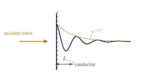
Fig. 304 A wave arriving at the flat surface of a conductor (hatched, filling \(z>0\)). Inside the metal the field is a travelling wave multiplied by the decaying envelope \(e^{-z/\delta}\) (dashed), where \(\delta\) is the skin depth of eq-wm-skin: at low frequency the real and imaginary parts of the refractive index are equal, so the wave attenuates over the same distance in which its phase advances by one radian. In copper \(\delta\) is 9.2 mm at 50 Hz and 65 µm at 1 MHz, which is why a mains conductor is solid metal and a radio-frequency one is a thin plated tube.#
σ (Drude, from n and τ) = 5.9670e+07 S/m vs measured 5.9600e+07 S/m
ħω_p (copper) = 10.807 eV
f δ (full Drude) δ = √(2/μ₀σω) ratio
5e+01 9.2142e-03 9.2142e-03 1.000000
1e+06 6.5154e-05 6.5154e-05 1.000000
1e+09 2.0602e-06 2.0604e-06 0.999921
the two expressions first differ by 1% at f = 1.41e+11 Hz
at λ = 633 nm (ωτ = 74.4): δ_Drude = 18.6 nm, √(2/μ₀σω) = 3.0 nm, ratio = 6.20
Validation 4#
✓ copper's Drude conductivity ne²τ/m reproduces the measured 5.96×10⁷ S/m [got 5.96699e+07 vs expected 5.96e+07 (rtol=0.02, atol=1e-09)]
✓ the full Drude skin depth equals √(2/μ₀σω) at 50 Hz and 1 MHz, where ωτ ≪ 1 [max|Δ| = 5.11713e-12 (rtol=0.0001, atol=1e-09)]
✓ the skin depth of copper at mains frequency is 9.2 mm [got 0.0092142 vs expected 0.0092 (rtol=0.01, atol=1e-09)]
✓ and 65 µm at 1 MHz: high-frequency current rides on the surface [got 6.51542e-05 vs expected 6.5e-05 (rtol=0.01, atol=1e-09)]
True
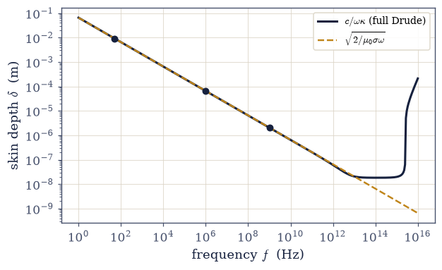
Fig. 305 The skin depth of copper over sixteen decades of frequency: the full Drude result \(\delta=c/\omega\kappa\) with \(\kappa=\operatorname{Im}\sqrt{\varepsilon_r}\) (dark) against the good-conductor formula \(\sqrt{2/\mu_0\sigma\omega}\) (amber, dashed). The two are indistinguishable across thirteen decades, from mains frequency (9.2 mm) through 1 MHz (65 µm) to 1 GHz (2.1 µm, marked points), and part company only when \(\omega\tau\) approaches one in the infrared, where the electron no longer collides many times per cycle. At the helium–neon wavelength the approximation is wrong by a factor of six.#
Exercise 5 — The plasma frequency: why metals shine and the ionosphere bounces radio (student)#
Push the Drude function Eq. 280 to the opposite extreme. When \(\omega\tau\gg1\) the electron completes many cycles between collisions, damping becomes irrelevant, and what remains is Eq. 282, \(\varepsilon_r=1-\omega_p^2/\omega^2\): real, no absorption, and negative for every \(\omega<\omega_p\). A negative \(\varepsilon_r\) gives a purely imaginary \(\tilde n=i\kappa\), so no wave propagates. Yet with \(n=0\) there is nothing to absorb either, and the energy that cannot go forward has only one place left to go. The metal reflects it all.
The mechanical picture behind \(\omega_p\) is worth having (Fig. 306). Displace the whole electron sea rigidly by \(u\) against its fixed positive background: one face of the slab is left with an uncompensated positive sheet, the other with an excess negative one, and the field between them, \(E=n e u/\varepsilon_0\), pulls the electrons back. That is a harmonic restoring force with \(\ddot u=-(ne^2/\varepsilon_0 m)u\), so the gas rings at exactly \(\omega_p\). The plasma frequency is not an abstraction fitted to a curve, it is the natural frequency of the electron gas as a whole.
Two materials make the point. Aluminium, with three valence electrons per atom (\(n=1.808\times10^{29}\,\mathrm{m^{-3}}\), \(\tau=8\,\)fs), has its \(\omega_p\) in the deep ultraviolet, so it is a mirror across the entire visible spectrum and turns transparent only above \(\sim16\,\)eV; the measured bulk plasmon energy is \(15.8\,\)eV. The night-time ionosphere, a far thinner gas at \(n_e=1\times10^{11}\,\mathrm{m^{-3}}\), has its \(\omega_p\) down in the megahertz, which is why an AM broadcast at 1 MHz reflects off the sky and can be heard a continent away while an FM signal at 100 MHz goes straight through to the satellites.
Part a) Compute \(\omega_p=\sqrt{ne^2/\varepsilon_0m}\) for aluminium and report \(\hbar\omega_p\) in eV against the measured \(15.8\,\)eV, and the corresponding vacuum wavelength \(\lambda_p=2\pi c/\omega_p\).
Part b) With the eps_drude you wrote in Exercise 4, at \(\tau=8\,\)fs, evaluate the
normal-incidence reflectance \(R=\bigl|(1-\tilde n)/(1+\tilde n)\bigr|^2\) — the
\(\theta_i=0\) case of Eq. 284, where the two polarizations coincide — on 1200
photon energies spaced linearly over \([1,\,30]\,\)eV, and plot it
(Fig. 307).
Part c) Repeat with the collisionless Eq. 282 and confirm with
numpy.allclose that \(R=1\) exactly (to \(10^{-12}\)) at every energy below
\(\hbar\omega_p\), and \(R<1\) above. Reflection without absorption is what a negative
\(\varepsilon_r\) means.
Part d) For the ionosphere compute \(f_p=\omega_p/2\pi\) and compare it with the radio engineer’s rule \(f_p=8.98\sqrt{n_e}\,\)Hz (\(n_e\) in \(\mathrm{m^{-3}}\)), then classify a 1 MHz AM carrier and a 100 MHz FM carrier as reflected or transmitted by evaluating the sign of \(\varepsilon_r\) at each.
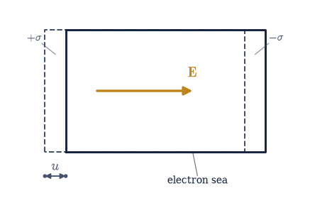
Fig. 306 Where the plasma frequency comes from. The electron sea of a metal (solid outline) is displaced rigidly by \(u\) relative to its fixed positive ion background (dashed outline), leaving an uncompensated positive sheet \(+\sigma=+neu\) on one face and an excess negative sheet \(-\sigma\) on the other. The field \(\mathbf E\) between them (amber) is uniform and restoring, giving \(\ddot u = -(ne^2/\varepsilon_0 m)\,u\): the gas oscillates at \(\omega_p=\sqrt{ne^2/\varepsilon_0 m}\). Below that frequency an incident wave finds \(\varepsilon_r<0\), cannot propagate, and is reflected in full.#
aluminium: ħω_p = 15.789 eV vs measured 15.8 eV
λ_p = 78.5 nm (deep ultraviolet)
R at 2 eV (visible) = 0.9896
R at 20 eV = 0.0571
collisionless: R = 1 to 1e-12 for every ω < ω_p: True; R < 1 above: True
ionosphere (n_e = 1e+11 m⁻³): f_p = 2.839 MHz
8.98√n_e = 2.840 MHz
AM 1 MHz: ε_r = -7.062 → reflected (ε_r < 0)
FM 100 MHz: ε_r = +0.999 → transmitted (ε_r > 0)
Validation 5#
✓ aluminium's computed plasma energy ħ√(ne²/ε₀m) matches the measured 15.8 eV [got 15.7891 vs expected 15.8 (rtol=0.01, atol=1e-09)]
✓ a collisionless electron gas reflects perfectly (R = 1 to 1e-12) below ω_p and transmits above it: negative ε_r means reflection without absorption
✓ the ionospheric plasma frequency agrees with the radio rule f_p = 8.98√n_e Hz [got 2.8393e+06 vs expected 2.83973e+06 (rtol=0.001, atol=1e-09)]
True
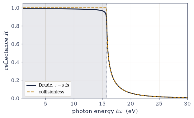
Fig. 307 Why aluminium is a mirror. The normal-incidence reflectance \(R=|(1-\tilde n)/(1+\tilde n)|^2\) of a Drude free-electron gas with aluminium’s parameters (\(n=1.808\times10^{29}\,\mathrm{m^{-3}}\), \(\tau=8\) fs, dark curve) stays above \(0.97\) from the infrared through the visible and collapses at the plasma energy \(\hbar\omega_p=15.79\) eV (dotted vertical): below it \(\varepsilon_r<0\) and no wave can propagate, above it the metal is a window. The collisionless limit (amber, dashed) makes the statement exact, with \(R=1\) to machine precision everywhere below \(\omega_p\). The shaded region is where \(\varepsilon_r<0\).#
Exercise 6 — Snell’s law is phase matching (worked)#
Everything so far has happened inside one uniform material. Put two of them face to face and the question becomes what a wave does at the boundary (Fig. 308). The answer divides cleanly in two, and the first half needs no amplitudes at all.
The boundary conditions of §3.13 — \(E_\parallel\) continuous, \(H_\parallel\) continuous — are not conditions at one point. They must hold at every point \(x\) of the interface and at every time \(t\). The incident, reflected and transmitted waves carry the phase factors \(e^{i(k_{1x}x-\omega_i t)}\), \(e^{i(k_{rx}x-\omega_r t)}\) and \(e^{i(k_{tx}x-\omega_t t)}\), and a sum of such factors can vanish for all \(x\) and all \(t\) only if the factors are identical. Hence one frequency for all three, and one tangential wavevector: \(k_1\sin\theta_i=k_1\sin\theta_r=k_2\sin\theta_t\) with \(k_j=n_j\omega/c\), which is Eq. 283. Reflection angle equals incidence angle, and \(n_1\sin\theta_i=n_2\sin\theta_t\). Snell’s law is not an empirical rule about rays; it is what “for all \(x\)” means.
That argument can be measured rather than asserted. Take the incident wave’s variation along the interface, \(e^{ik_1\sin\theta_i x}\), and a trial transmitted variation \(e^{ik_2\sin\theta_t x}\) at an assumed angle \(\theta_t\), and compute how badly they fail to match over a stretch of the surface,
For any \(\theta_t\) but one, the two run out of step and \(M\) is of order \(2\); at Snell’s angle it is exactly zero, and stays zero however long the interface.
The interface here is air to glass, \(n_1=1\) and \(n_2=1.5\) (the static index computed in Exercise 3), at vacuum wavelength \(\lambda=633\,\)nm and incidence angle \(\theta_i=40^\circ\); the matching stretch is \(L=20\lambda\).
Part a) Build \(M(\theta_t)\) with numpy.trapezoid on 20001 sample points across
\([0,L]\), evaluate it on 1801 trial angles spaced linearly over \([0^\circ,89.9^\circ]\), and
plot it (Fig. 309). Report \(M\) at the minimum and at
\(\theta_t\pm2^\circ\).
Part b) Locate the transmitted angle as the root of the tangential-wavevector mismatch
\(g(\theta_t)=k_1\sin\theta_i-k_2\sin\theta_t\) with scipy.optimize.brentq bracketed on
\([0,\pi/2]\) (the function is monotone there, so the bracket is safe), and compare it with
\(\arcsin(n_1\sin\theta_i/n_2)=25.374^\circ\).
Part c) Apply the same matching within medium 1, where the reflected wave has the same \(|k|\) as the incident one, so \(\sin\theta_r=\sin\theta_i\); confirm the reflected angle equals \(40^\circ\).
Part d) Reverse the media to glass into air. Show that \(g\) has no root once
\(\sin\theta_i>n_2/n_1\) (evaluate its sign at both bracket ends), and locate the critical
angle as the root of \(n_1\sin\theta-n_2\) with scipy.optimize.brentq on
\([0,\pi/2]\): \(\theta_c=\arcsin(n_2/n_1)=41.810^\circ\), the gateway to Exercise 9.
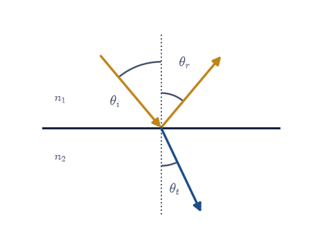
Fig. 308 The interface geometry that the rest of the notebook works on. A plane wave in medium 1 (index \(n_1\)) strikes a flat boundary at the angle of incidence \(\theta_i\), measured from the normal (dotted). Part of it is reflected at \(\theta_r\) and part transmitted into medium 2 (index \(n_2>n_1\)) at \(\theta_t\). Requiring the boundary conditions to hold at every point of the surface forces all three waves to share a tangential wavevector, which gives \(\theta_r=\theta_i\) and \(n_1\sin\theta_i=n_2\sin\theta_t\): the law of reflection and Snell’s law, obtained before any amplitude is written down. The angles drawn are the worked case \(\theta_i=40^\circ\), \(\theta_t=25.4^\circ\) for air into glass.#
M at Snell's angle = 0.000e+00
M two degrees either side = 2.095, 2.129
θ_t (brentq) = 25.373994° vs arcsin(n₁sinθ_i/n₂) = 25.373994°
θ_r (brentq) = 40.000000° vs θ_i = 40.000000°
glass→air at 60°: mismatch stays positive across the whole bracket (1.299 → 0.299) — no real θ_t
θ_c (brentq) = 41.810315° vs arcsin(n₂/n₁) = 41.810315°
Validation 6#
✓ phase matching gives Snell's law: the mismatch root is arcsin(n₁sinθ_i/n₂) = 25.374° [got 0.44286 vs expected 0.44286 (rtol=1e-09, atol=1e-09)]
✓ and the law of reflection, θ_r = θ_i = 40° [got 0.698132 vs expected 0.698132 (rtol=1e-09, atol=1e-09)]
✓ the interface mismatch vanishes at Snell's angle [got 0 vs expected 0 (rtol=1e-06, atol=1e-12)]
✓ and is of order unity two degrees away: only one angle matches phases along the surface [M(θ_t ± 2°) = 2.095, 2.129]
✓ glass into air at 60° has no real refraction angle at all
✓ the critical angle for glass into air is arcsin(n₂/n₁) = 41.810° [got 0.729728 vs expected 0.729728 (rtol=1e-09, atol=1e-09)]
True
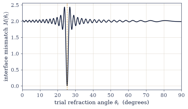
Fig. 309 Snell’s law located by measurement rather than quoted. The mean-square failure \(M(\theta_t)\) of a trial transmitted wave \(e^{ik_2\sin\theta_t x}\) to match the incident variation \(e^{ik_1\sin\theta_i x}\) over \(20\) wavelengths of interface, for air into glass at \(\theta_i=40^\circ\). Away from one special angle the two run out of step and \(M\) hovers near \(2\); at \(\theta_t=25.374^\circ\) (amber dotted) it drops to zero, and it is exactly zero there however long the interface is taken to be. The oscillations either side are the finite-length beating between the two phase factors.#
Exercise 7 — The Fresnel relations, from two continuity conditions (student)#
Phase matching fixed the directions; the amplitudes need the boundary conditions themselves. With no free surface charge and no free surface current, the conditions of §3.13 say that the components of \(\mathbf E\) and of \(\mathbf H\) lying in the interface are continuous across it. Two conditions, two unknowns (the reflected and transmitted amplitudes, in units of the incident one), and the answer depends on which way the field points relative to the plane of incidence — the plane containing the incident ray and the normal, drawn in Fig. 308.
For s-polarization \(\mathbf E\) is perpendicular to that plane, so it lies entirely in the interface and continuity of \(E_\parallel\) reads \(1+r_s=t_s\); the accompanying \(\mathbf H\) lies in the plane of incidence, its tangential component picks up a \(\cos\theta\), and with \(H=nE/\mu_0c\) its continuity reads \(n_1\cos\theta_i\,(1-r_s)=n_2\cos\theta_t\,t_s\) (the minus sign because the reflected wave’s \(\mathbf H\) has reversed). For p-polarization the roles swap: \(\mathbf H\) is perpendicular to the plane of incidence and gives \(n_1(1+r_p)=n_2t_p\), while \(\mathbf E\) lies in it and gives \(\cos\theta_i\,(1-r_p)=\cos\theta_t\,t_p\). Each pair is a \(2\times2\) linear system, and solving it is the derivation of the Fresnel relations Eq. 284 and Eq. 285.
What a detector reports is not the amplitude but the power. The reflectance is \(R=|r|^2\), while the transmittance carries a geometric factor, \(T=(n_2\cos\theta_t/n_1\cos\theta_i)\,|t|^2\), because the refracted beam has a different cross-section and travels at a different speed. Energy conservation is then the single statement \(R+T=1\), which the coefficients must satisfy at every angle without having been asked to.
The interface is again air to glass, \(n_1=1\), \(n_2=1.5\).
Part a) Write fresnel_s(n1, n2, theta_i): form \(\cos\theta_t\) from
Eq. 283 as numpy.sqrt(1 - (n1*sin(theta_i)/n2)**2 + 0j) (complex, so that
Exercise 9 can reuse it unchanged past the critical angle), assemble the \(2\times2\)
coefficient matrix and right-hand side of the two s-polarization conditions above as an
explicit numpy array, and solve with numpy.linalg.solve for \((r_s,t_s)\). Writing the
rows means deciding which condition supplies which row and where each \(\cos\theta\) and
each \(n\) belongs. Write this one yourself — the implementation is the lesson.
Part b) The same for fresnel_p(n1, n2, theta_i) from the p-polarization pair.
Part c) Evaluate both on 1801 angles spaced linearly over \([0^\circ,89.9^\circ]\) and
compare with the closed forms Eq. 284 and Eq. 285 using
numpy.allclose.
Part d) Form \(R=|r|^2\) and \(T=(n_2\cos\theta_t/n_1\cos\theta_i)|t|^2\) for both polarizations, plot them (Fig. 310), confirm \(R+T=1\) at every angle, and report the normal-incidence value against \(((n_1-n_2)/(n_1+n_2))^2=0.04\): a window pane reflects four percent per surface, which is why a shop window at night is a mirror.
solved coefficients match eq-wm-fresnel-s and eq-wm-fresnel-p: True
max |R_s + T_s − 1| = 4.44e-16
max |R_p + T_p − 1| = 6.66e-16
normal incidence: R_s = 0.040000, R_p = 0.040000, ((n₁−n₂)/(n₁+n₂))² = 0.040000
Validation 7#
✓ the 2×2 boundary-condition system reproduces the Fresnel relations at every angle
✓ energy is conserved for s-polarization: R + T = 1 at every angle of incidence [max|Δ| = 4.44089e-16 (rtol=1e-12, atol=1e-09)]
✓ and for p-polarization [max|Δ| = 6.66134e-16 (rtol=1e-12, atol=1e-09)]
✓ at normal incidence both polarizations give R = ((n₁−n₂)/(n₁+n₂))² = 0.04 [got 0.04 vs expected 0.04 (rtol=1e-12, atol=1e-09)]
True
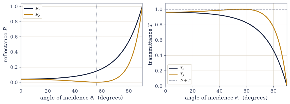
Fig. 310 The Fresnel relations for air into glass (\(n_1=1\), \(n_2=1.5\)), obtained by solving the \(2\times2\) boundary-condition system at each angle. Left: the reflectances \(R_s\) (dark) and \(R_p\) (amber), equal at normal incidence at the familiar \(4\%\), diverging as the angle opens, and both going to \(1\) at grazing incidence. \(R_p\) touches zero at Brewster’s angle \(56.31^\circ\) (dotted vertical), where the reflected light is purely s-polarized. Right: the transmittances, each the complement of its reflectance. The dashed line is \(R+T\) for both polarizations, flat at \(1\) to \(10^{-15}\): nothing was assumed about energy, and energy came out conserved.#
Exercise 8 — Brewster’s angle (student)#
One line of Eq. 285 deserves its own exercise. The numerator of \(r_p\) is \(n_2\cos\theta_i-n_1\cos\theta_t\), and there is an angle where it vanishes outright: the p-polarized reflection disappears. Combining that condition with Snell’s law Eq. 283 gives Brewster’s angle Eq. 286, \(\tan\theta_B=n_2/n_1\), equivalently \(\theta_B+\theta_t=90^\circ\).
The second form is the one to keep, because it says why (Fig. 311). The reflected wave is not a wave that bounced; it is radiation emitted by the charges the transmitted wave drives in the second medium. For p-polarization those charges oscillate in the plane of incidence, perpendicular to the refracted ray, so when \(\theta_B+\theta_t=90^\circ\) the direction the reflected ray would take is along the dipoles’ own axis. A dipole radiates as \(\sin^2\Theta\) from its axis (§3.10) and therefore radiates nothing there at all. The reflection has no source. Light reflected off water or glass near \(\theta_B\) is consequently pure s-polarization, which is exactly what a polarizing filter is turned to block.
The interface is air to glass, \(n_1=1\), \(n_2=1.5\), on the coefficients built in Exercise 7.
Part a) Locate the zero of \(\operatorname{Re}r_p(\theta_i)\) with
scipy.optimize.brentq bracketed on \([30^\circ,80^\circ]\), using the fresnel_p you
wrote in Exercise 7, and compare with \(\arctan(n_2/n_1)=56.310^\circ\).
Part b) Compute \(\theta_t\) at that angle from Eq. 283 and confirm \(\theta_B+\theta_t=90^\circ\).
Part c) Form the degree of polarization of the reflected light, \(P=(R_s-R_p)/(R_s+R_p)\), on the angle grid of Exercise 7, plot it (Fig. 312), and confirm \(P=1\) at \(\theta_B\): at that one angle the reflection is completely polarized.
Part d) Repeat Part a for glass to air (\(n_1=1.5\), \(n_2=1\)) and check that the two Brewster angles are complementary, \(\arctan(1/1.5)=33.690^\circ=90^\circ-56.310^\circ\), which is the same geometric statement seen from the other side of the glass.
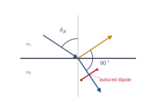
Fig. 311 Why the p-polarized reflection vanishes at Brewster’s angle. At \(\theta_B=56.31^\circ\) for air into glass the reflected ray (amber) and the refracted ray (blue) leave the interface exactly \(90^\circ\) apart. The refracted wave drives the charges of the second medium into oscillation perpendicular to its own direction of travel, so for p-polarization the induced dipole (double-headed arrow) points precisely along the direction the reflected ray would take. A dipole radiates as \(\sin^2\Theta\) measured from its axis and so emits nothing along it: the reflection has no source, and what light does come back is purely s-polarized.#
Brewster (brentq) = 56.309932° vs arctan(n₂/n₁) = 56.309932°
θ_B + θ_t = 90.000000000°
degree of polarization at the grid point nearest θ_B: P = 0.999999
R_p there = 5.602e-08 (R_s = 0.1478)
glass→air Brewster = 33.690068° (90° − 56.310° = 33.690068°)
Validation 8#
✓ the zero of r_p sits at Brewster's angle arctan(n₂/n₁) = 56.310° [got 0.982794 vs expected 0.982794 (rtol=1e-09, atol=1e-09)]
✓ there the reflected and refracted rays are exactly perpendicular, θ_B + θ_t = 90° [got 1.5708 vs expected 1.5708 (rtol=1e-09, atol=1e-09)]
✓ so the reflected light is completely s-polarized: the degree of polarization is 1 [got 0.999999 vs expected 1 (rtol=0.0001, atol=1e-09)]
✓ and the glass-to-air Brewster angle is its complement, 33.690° [got 0.588003 vs expected 0.588003 (rtol=1e-09, atol=1e-09)]
True
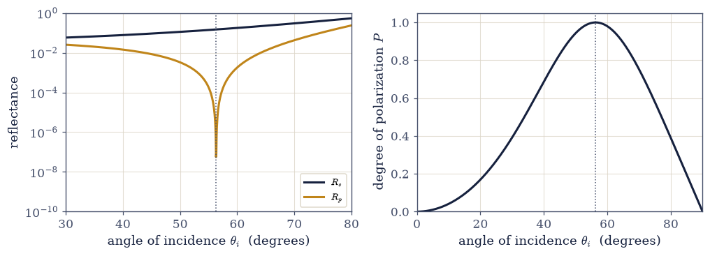
Fig. 312 Brewster’s angle at work, for air into glass. Left: the two reflectances near \(\theta_B\) on a logarithmic scale — \(R_s\) (dark) rises smoothly while \(R_p\) (amber) plunges to zero at \(56.310^\circ\) (dotted vertical), limited here only by the angular sampling. Right: the degree of polarization \(P=(R_s-R_p)/(R_s+R_p)\) of the reflected light, which reaches exactly \(1\) at \(\theta_B\): every photon that comes back at that angle is polarized perpendicular to the plane of incidence. Rotating a polarizing filter to block that direction removes the glare from water, glass, and wet roads.#
Exercise 9 — Total internal reflection and the evanescent wave (student)#
Send the light the other way, from glass into air, and Exercise 6 already showed what goes wrong: past \(\theta_c=\arcsin(n_2/n_1)=41.810^\circ\) the phase-matching condition Eq. 283 has no real solution. Nothing breaks, though. Write \(\cos\theta_t=\sqrt{1-(n_1\sin\theta_i/n_2)^2}\) as a complex number and it becomes \(i\,q\) with \(q=\sqrt{(n_1\sin\theta_i/n_2)^2-1}\) real, the Fresnel formulas Eq. 284 and Eq. 285 carry straight through, and the transmitted wave turns into the evanescent field Eq. 287: a disturbance that runs along the surface with the incident wave’s tangential wavevector and dies exponentially away from it over the penetration depth \(d=\lambda/2\pi\sqrt{n_1^2\sin^2\theta_i-n_2^2}\) (Fig. 313).
Three things about that field are worth measuring rather than believing. Both reflection coefficients acquire modulus exactly one, so the reflection is total — better than any metal mirror, which is why an optical fibre is glass and not silver. Each acquires a phase, and the phases differ between the two polarizations, which is how a glass prism with no coating on it can be made into a quarter-wave plate. And the field on the far side is not small: at \(45^\circ\) its amplitude exceeds the incident one, while the time-averaged energy flux normal to the interface, \(\langle S_z\rangle=|E_t|^2 \operatorname{Re}\tilde k_z/2\mu_0\omega\), is exactly zero because \(\tilde k_z\) is purely imaginary. A large field that transports nothing across the boundary is what “total” means. Bring a second glass surface within a few hundred nanometres and the decay is cut short before it finishes: light crosses the gap, an optical tunnelling that is the working principle of the fingerprint sensor on a phone.
The interface is glass to air, \(n_1=1.5\), \(n_2=1\), at \(\lambda=633\,\)nm, using the
fresnel_s and fresnel_p you built in Exercise 7, which already keep \(\cos\theta_t\)
complex.
With your assistant
Part e wants an animation of the field on both sides of the interface: two half-spaces
on one grid, a frame index, an imshow whose array is refreshed each frame. That
scaffolding is generic and a reasonable thing to have generated for you. The physics
inside it is not. Check yourself that the field your animation draws above the interface
decays with the penetration depth \(d\) of Eq. 287, by fitting \(\ln|E|\)
against \(z\) with numpy.polyfit and comparing the slope with \(-1/d\). The check is yours.
Part a) Evaluate fresnel_s and fresnel_p on 801 angles spaced linearly over
\([\theta_c+0.01^\circ,\,89.9^\circ]\) and confirm with numpy.allclose that
\(|r_s|=|r_p|=1\) to \(10^{-12}\): past the critical angle no power at all crosses the
boundary.
Part b) Take the reflection phases with numpy.angle and compare them with the
closed forms \(\delta_s=-2\arctan(q'/\cos\theta_i)\) and
\(\delta_p=-2\arctan\bigl((n_1/n_2)^2q'/\cos\theta_i\bigr)\), where
\(q'=\sqrt{\sin^2\theta_i-(n_2/n_1)^2}\). Then find the angle at which the difference
\(\delta_p-\delta_s\) is largest, with numpy.argmax over the grid. It peaks just above
\(45^\circ\) at slightly more than \(45^\circ\) of phase difference, which is why two
internal reflections in a suitably cut glass block (a Fresnel rhomb) turn linear
polarization into circular with no coating at all.
Part c) Compute the penetration depth \(d\) of Eq. 287 across the same grid, and report it at \(45^\circ\) and \(60^\circ\).
Part d) At \(\theta_i=45^\circ\) report \(|t_s|^2\), and evaluate the normal energy flux \(\langle S_z\rangle\propto\operatorname{Re}\tilde k_z\) with \(\tilde k_z=(2\pi n_2/\lambda)\cos\theta_t\), together with the along-surface flux \(\langle S_x\rangle\propto\operatorname{Re}\tilde k_x\). The first is zero and the second is not: the evanescent field carries energy along the interface and none across it.
Part e) Animate the total field on a grid spanning \(x\in[0,3]\,\mu\)m and \(z\in[-1.2,0.9]\,\mu\)m over one optical period (Fig. 314): in the glass the sum \(e^{i(k_xx+k_zz-\omega t)}+r_se^{i(k_xx-k_zz-\omega t)}\), in the air the evanescent \(t_se^{ik_xx}e^{-z/d}e^{-i\omega t}\).
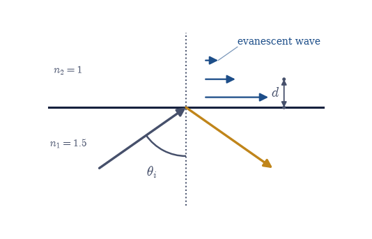
Fig. 313 Total internal reflection at a glass–air boundary. A ray inside the glass (\(n_1=1.5\)) strikes the surface at \(\theta_i>\theta_c=41.81^\circ\), and since \(n_1\sin\theta_i>n_2\) there is no real refraction angle: the whole beam is reflected (amber). The field beyond the surface does not vanish, though. It becomes the evanescent wave, travelling along the interface with the incident tangential wavevector and decaying away from it as \(e^{-z/d}\) (the shrinking arrows), with \(d=285\) nm at \(\theta_i=45^\circ\) for \(\lambda=633\) nm. It carries no energy across the boundary.#
|r_s| = 1 to 1e-12: True; |r_p| = 1 to 1e-12: True
computed phases match the closed forms: True
largest |δ_p − δ_s| = 45.24° at θ_i = 51.68° (the Fresnel rhomb)
penetration depth: 284.7 nm at 45°, 121.6 nm at 60°
at 45°: |t_s|² = 3.6000 (the field beyond the surface is the larger one)
k̃_z = 0.0000e+00+3.5094e+06j 1/m → ⟨S_z⟩ ∝ Re k̃_z = 0.000e+00
k̃_x = 1.0528e+07 1/m → ⟨S_x⟩ ∝ Re k̃_x = 1.053e+07 (energy runs along the surface)
Validation 9#
✓ beyond the critical angle both Fresnel coefficients have modulus one: the reflection is total for either polarization
✓ and their phases match the closed-form total-reflection phases
✓ the evanescent field penetrates 285 nm into the air at 45° for λ = 633 nm [got 2.847e-07 vs expected 2.847e-07 (rtol=0.001, atol=1e-09)]
✓ yet it carries no energy across the boundary: Re k̃_z = 0, so ⟨S_z⟩ = 0 [got 0 vs expected 0 (rtol=1e-06, atol=1e-12)]
✓ while the transmitted amplitude exceeds the incident one [|t_s|² = 3.6000]
True