2.9 Lagrange Points and the Restricted Three-Body Problem

Elementary Computational Physics

Volume II — Analytical Mechanics Notebook 2.9

Five points where a small body can ride along with two large ones: the effective potential of the rotating frame, the collinear and triangular equilibria, the mass-ratio threshold that makes L4 and L5 stable, and the tadpole orbits of the Trojan asteroids.

Level · advanced   •   Est. · 90–120 min

Raymond Amador v1.4.0  ·  2026-07-31  ·  CC BY 4.0 (text) / MIT (code)

Notebook overview

Three gravitating bodies have no general closed-form orbit: the three-body problem is the classic edge where analytical mechanics runs out of formulae and computation takes over. But one special case is both tractable and useful. Let two massive bodies (the primaries, say the Earth and the Moon) circle their common centre of mass, and watch a third body so light that it pulls on nobody. Where can that third body sit so that, seen from the rotating frame of the primaries, it does not move at all? There are exactly five such points, found by Euler and Lagrange, and they are not a curiosity: the James Webb Space Telescope parks at one of them, and thousands of Trojan asteroids librate around two more.

The trick that makes the five points visible is the one from §2.4, raised to two dimensions and given a twist. In the co-rotating frame the motion is governed by an effective potential Ω, the genuine gravity of the two primaries plus a centrifugal term from the rotation. Its stationary points are the equilibria, and we hunt them exactly as §2.4 hunted turning points: as roots, found with the bracket-discovering solver now living in ecp.mechanics. Whether each equilibrium is stable is a small-oscillation question (§2.7), with one beautiful surprise: the triangular points L4 and L5 are minima of Ω yet dynamically unstable (the rotating-frame force runs up the Ω-gradient), and the Coriolis force can still trap a body there, provided one primary is heavy enough relative to the other.

We will map Ω, locate all five points, settle their stability and the mass-ratio threshold that governs it, and then watch the payoff: a test mass started just off L4 traces a slow tadpole orbit instead of falling away, exactly as Jupiter’s Trojans do. That tadpole genuinely moves, so it earns an animation; the potential map, the point map, and the stability curve are static, as such things should be.

How to read the checks. Each exercise ends with a validate call against an independent fact: a finite-difference gradient, a vanishing force, an equilateral distance, a conserved Jacobi constant. A ✓ is strong evidence; a ✗ is a prompt to locate the discrepancy, not a verdict.

Scope. A working application, not a treatise on celestial mechanics. The standard references are Murray & Dermott, Solar System Dynamics [MD99], and Szebehely’s Theory of Orbits [Sze67]; the mechanics background is Nolting [Nol16a],[Nol16b].

Theory in brief

The restricted three-body problem

Two primaries of masses \(m_1 \ge m_2\) orbit their barycentre on circles; a third body of negligible mass moves in their combined gravity without affecting them. We work in the co-rotating frame in which the primaries are fixed, and nondimensionalise so that the total mass, the separation, and the angular velocity are all \(1\). With the mass ratio

\[ \mu = \frac{m_2}{m_1 + m_2}, \qquad 0 < \mu \le \tfrac12, \]

the heavier primary (mass \(1-\mu\)) sits at \((-\mu, 0)\) and the lighter (mass \(\mu\)) at \((1-\mu, 0)\). The Earth–Moon system, our running example, has \(\mu = 0.01215\).

The effective potential

In the rotating frame the planar motion obeys (Murray & Dermott [MD99], ch. 3, derive the frame transformation in full)

(173)\[\ddot x - 2\dot y = \frac{\partial\Omega}{\partial x}, \qquad \ddot y + 2\dot x = \frac{\partial\Omega}{\partial y}, \qquad \Omega(x,y) = \tfrac12\big(x^2+y^2\big) + \frac{1-\mu}{r_1} + \frac{\mu}{r_2},\]

where \(r_1, r_2\) are the distances to the two primaries. The \(\tfrac12(x^2+y^2)\) term is the centrifugal contribution of the rotating frame and the other two are gravity; the \(2\dot y\), \(2\dot x\) terms are the Coriolis force, which depends on the velocity and so does no work. Equilibria of the rotating-frame motion are the stationary points \(\nabla\Omega = 0\): this is the effective potential of §2.4, now in two dimensions and carrying a centrifugal term.

The five Lagrange points

Solving \(\nabla\Omega = 0\) (Eq. 173) gives five equilibria (Eq. 174). Three are collinear, on the \(y=0\) axis where \(\partial\Omega/\partial x = 0\): \(L_1\) between the primaries, \(L_2\) beyond the lighter one, \(L_3\) beyond the heavier one. Two are triangular, \(L_4\) and \(L_5\), forming equilateral triangles with the primaries at

(174)\[L_{4,5} = \left(\tfrac12 - \mu,\ \pm\tfrac{\sqrt3}{2}\right),\]

each a unit distance from both primaries.

Stability and the Routh criterion

Linearising the rotating-frame equations about a Lagrange point gives a small- oscillation problem (§2.7) with a twist: the Hessian of \(\Omega\) supplies the restoring terms and the Coriolis force couples the coordinates. The collinear points are saddles, hence unstable. The triangular points are stable only when the primaries are lopsided enough, the Routh criterion (Exercise 5 traces the threshold numerically; Murray & Dermott [MD99] carry the linearisation to the closed form)

(175)\[\mu < \mu_{\rm crit} = \tfrac12\Big(1 - \sqrt{\tfrac{23}{27}}\Big) \approx 0.0385, \qquad \text{equivalently}\quad \frac{m_1}{m_2} > 24.96 .\]

What makes this surprising is that \(L_4\) and \(L_5\) are minima of \(\Omega\), yet unstable: the rotating-frame acceleration runs up the gradient (\(+\nabla\Omega\)), so with no rotation a body rolls off. The velocity-dependent Coriolis force curves its path back, trapping it, provided the mass ratio clears the threshold.

The Jacobi constant

The rotating frame does work, so energy is not conserved; but the combination

(176)\[C = 2\Omega(x,y) - v^2, \qquad v^2 = \dot x^2 + \dot y^2,\]

is. This Jacobi constant is the one integral of motion of the problem, and the curve \(2\Omega = C\) (zero velocity) bounds the region the test body can reach.

Beyond gravity

“Equilibrium in the effective potential of a rotating or interacting system” is a general idea, not only a gravitational one. The same stationary-point-plus-Hessian stability analysis locates equilibrium configurations and transition states on molecular potential-energy surfaces, and governs many-body equilibria more broadly (a forward link to the later volumes). Here it is gravity, with two famous hooks: JWST parks at the Sun–Earth \(L_2\), and Jupiter’s Trojan asteroids occupy its \(L_4\) and \(L_5\).

Setup

Setup holds the data — the Earth–Moon mass ratio \(\mu\), the closed-form triangular points Eq. 174 — together with the imports and a single instrument, the positions of the two primaries in the rotating frame. The notebook’s own machinery is not here: you build the effective potential \(\Omega\) with its gradient and Hessian in Exercise 1, the linear-stability matrix in Exercise 4, the co-rotating equations of motion in Exercise 6, and the Jacobi constant in Exercise 7.

The Setup below holds this notebook’s data and instruments — nothing you are asked to build. It is collapsed so the building stays yours; expand it whenever you want the details.

Show code cell source

Hide code cell source

import numpy as np
import sympy as sp
import matplotlib.pyplot as plt
from matplotlib.animation import FuncAnimation
from scipy.integrate import solve_ivp

from ecp import validate
from ecp.animate import show
from ecp.mechanics import bracketed_roots

MU = 0.01215  # data: Earth–Moon-like mass ratio, the running example

# data: the triangular points in closed form (eq-lagrange), evaluated at this μ
L4_POINT = np.array([0.5 - MU, np.sqrt(3) / 2.0])
L5_POINT = np.array([0.5 - MU, -np.sqrt(3) / 2.0])


# instrument: pure bookkeeping for the figures and the distance checks — the two
# positions are fixed by the nondimensionalisation itself (heavier at −μ, lighter
# at 1−μ), not derived by anything in this notebook.
def primaries(mu=MU):
    """Positions of the two primary masses in the rotating frame.

    The heavier at (−μ, 0) and lighter at (1−μ, 0), the fixed sources of the
    effective potential.

    Parameters
    ----------
    mu : float, optional
        Mass ratio (default the module value).

    Returns
    -------
    tuple of numpy.ndarray
        The two primary positions.
    """
    return np.array([-mu, 0.0]), np.array([1.0 - mu, 0.0])

Exercise 1 — The effective potential of the rotating frame

Before locating anything we need the landscape itself. The effective potential Eq. 173 is the landscape whose gradient drives the rotating-frame motion: two towering gravitational spikes at the primaries (where \(\Omega\to+\infty\)), and a centrifugal rise that grows like \(\tfrac12 r^2\) far out. A rotating-frame “potential” makes sense precisely because the Coriolis force does no work, so only Ω sets where the body can rest.

Everything that follows — the five points, their stability, the tadpole orbit, the Jacobi constant — is read off this one surface and its first two derivatives, so they had better be exact. Building \(\Omega\) symbolically and differentiating it with SymPy (the §2.1 habit) makes them so: no hand-differentiation slips, and sympy.lambdify turns the results into fast NumPy callables afterwards.

Part a) Write the effective potential of the co-rotating frame as SymPy expressions in \((x, y, \mu)\): the distance \(r_1\) to the heavier primary at \((-\mu, 0)\), the distance \(r_2\) to the lighter one at \((1-\mu, 0)\), then \(\Omega\) itself Eq. 173, and its first and second derivatives with sympy.diff. Lambdify the three into Omega(x, y, mu), grad_Omega(x, y, mu) returning \([\Omega_x, \Omega_y]\), and hessian_Omega(x, y, mu) returning the \(2\times2\) matrix of second derivatives. Write this one yourself — the implementation is the lesson: this single surface is the restricted three-body problem, and every later exercise is a question asked of it.

Part b) Certify the analytic gradient against central finite differences of \(\Omega\) (step \(h=10^{-6}\)) at a generic, non-equilibrium point, \((x,y)=(0.6,0.3)\).

Part c) Map \(\Omega\) for \(\mu = 0.01215\) (Fig. 160).

analytic ∇Ω at (0.6,0.3) = [-1.26878643 -0.66635565]
finite-difference ∇Ω      = [-1.26878643 -0.66635565]
max |Δ| = 9.91e-11

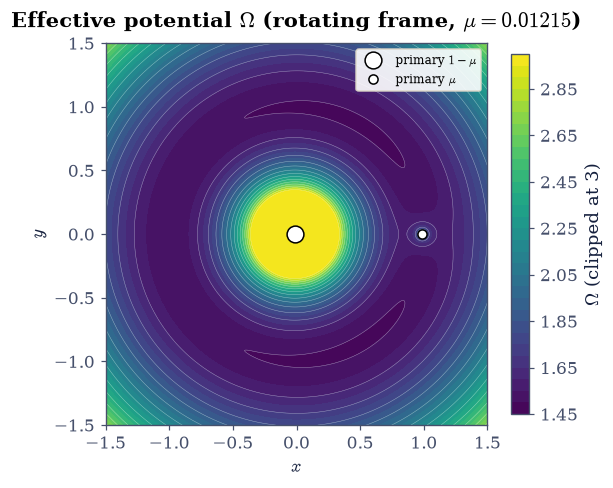
Fig. 160 The effective potential \(\Omega(x,y)=\frac12(x^2+y^2)+(1-\mu)/r_1+\mu/r_2\) of the rotating frame for \(\mu=0.01215\) (Earth–Moon), as filled contours (values clipped at 3 for visibility). Two towering gravitational spikes rise at the primaries (white markers, the larger at \((-\mu,0)\)); far out the centrifugal \(\frac12 r^2\) term lifts the surface. The five Lagrange points are the stationary points of this landscape, located in the next exercises.

Validation 1

✓  the analytic gradient of Ω matches finite differences   [max|Δ| = 9.90608e-11 (rtol=1e-06, atol=1e-09)]

True

Exercise 2 — The collinear points L1, L2, L3 (worked)

On the axis \(y = 0\) the problem collapses to one dimension: a Lagrange point is a root of \(\partial\Omega/\partial x = 0\) (Eq. 174). The function has poles at the two primaries, so we search three clean intervals (between the primaries, beyond the lighter, beyond the heavier) and let ecp.mechanics.bracketed_roots (which scans each interval on a fine sub-grid for sign changes, then refines each bracket) do the rest, a direct callback to the turning-point search of §2.4. The axial gradient we hand it is the grad_Omega you built in Exercise 1, restricted to \(y = 0\).

L1 x = 0.8369   (∂Ω/∂x = 1.26e-13)
L2 x = 1.1557   (∂Ω/∂x = 0.00e+00)
L3 x = -1.0051   (∂Ω/∂x = 6.88e-15)

Validation 2

✓  L1, L2, L3 are stationary points of Ω   [max|Δ| = 1.25677e-13 (rtol=1e-06, atol=1e-09)]

True

Exercise 3 — The triangular points L4, L5 are equilateral

The remaining two equilibria sit off the axis. The claim is that \(L_{4,5} = (\tfrac12-\mu,\ \pm\tfrac{\sqrt3}{2})\) (Eq. 174) are stationary and that each is a unit distance from both primaries, so the body and the two primaries form an equilateral triangle. This is exact for any \(\mu\).

Part a) Confirm numerically that \(\nabla\Omega\) vanishes at \(L_4\) and that \(r_1 = r_2 = 1\) there, using the grad_Omega you built in Exercise 1 and the Setup’s closed-form L4_POINT.

Part b) Mark all five points on the potential map (Fig. 161).

L4 = [0.48785   0.8660254]
distances to primaries: r1 = 1.000000, r2 = 1.000000  (both should be 1)
∇Ω at L4 = [-5.55111512e-17 -1.11022302e-16]  (should vanish)

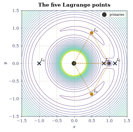
Fig. 161 The five Lagrange points of the Earth–Moon system (\(\mu=0.01215\)) on the effective-potential contours. The three collinear points \(L_1,L_2,L_3\) lie on the axis between and beyond the primaries; the triangular points \(L_4,L_5\) (amber) each form an equilateral triangle with the two primaries (dashed), a unit distance from both. \(L_1\)–\(L_3\) are saddles; \(L_4,L_5\) are effective-potential minima, unstable on their own but held in place by the Coriolis force.

Validation 3

✓  L4 forms an equilateral triangle with the primaries (unit distances)   [max|Δ| = 1.11022e-16 (rtol=1e-09, atol=1e-09)]
✓  ∇Ω vanishes at L4 (it is an equilibrium)   [max|Δ| = 1.11022e-16 (rtol=1e-06, atol=1e-12)]

True

Exercise 4 — Stability I: the collinear saddles

Knowing where the points are says nothing about whether a body stays there. We settle that the way §2.7 settled small oscillations: linearise the motion about the point and read off the eigenvalues. The rotating-frame linearisation carries the Hessian of \(\Omega\) plus the Coriolis coupling, giving a \(4\times4\) system. A purely imaginary spectrum means oscillation (stable); any eigenvalue with a positive real part means runaway growth (unstable).

Written out for the deviation \(\delta\mathbf{s} = (\delta x, \delta y, \delta\dot x, \delta\dot y)\) from an equilibrium, Eq. 173 linearises to \(\delta\dot{\mathbf{s}} = A\,\delta\mathbf{s}\) with

\[\begin{split} A = \begin{pmatrix} 0 & 0 & 1 & 0 \\ 0 & 0 & 0 & 1 \\ \Omega_{xx} & \Omega_{xy} & 0 & 2 \\ \Omega_{xy} & \Omega_{yy} & -2 & 0 \end{pmatrix}, \end{split}\]

the top two rows merely restating that \(\delta\dot x\) and \(\delta\dot y\) are the velocities, the bottom two carrying the Hessian of \(\Omega\) (the restoring terms) and the Coriolis coupling \(+2\delta\dot y\), \(-2\delta\dot x\).

Part a) Write stability_eigenvalues(x0, y0, mu): assemble that \(4\times4\) matrix from the hessian_Omega you built in Exercise 1 and return its four eigenvalues from numpy.linalg.eigvals. Write this one yourself — the implementation is the lesson: this matrix is exactly where the velocity-dependent Coriolis force enters the stability question, and Exercise 5 turns the same four numbers into the Routh threshold.

Part b) Apply it at \(L_1\) and show that one eigenvalue has a positive real part: the collinear points are saddles.

eigenvalues at L1:
   +2.9320+0.0000j
   -2.9320+0.0000j
   +0.0000+2.3344j
   +0.0000-2.3344j
max real part = 2.9320  (> 0 ⇒ unstable saddle)

Validation 4

✓  the collinear point L1 is linearly unstable (a saddle)   [max Re(λ) = 2.9320]

True

Exercise 5 — Stability II: the triangular points and the Routh criterion

This is the centrepiece, and the surprise. \(L_4\) and \(L_5\) are minima of \(\Omega\) — but the rotating-frame force runs up the \(\Omega\)-gradient, so drop a body there with the rotation switched off and it rolls away. Yet with rotation the velocity-dependent Coriolis force bends its path into a closed loop, provided the primaries are lopsided enough. The threshold is the Routh criterion Eq. 175, \(\mu_{\rm crit} = \tfrac12(1-\sqrt{23/27}) \approx 0.0385\), equivalently a mass ratio \(m_1/m_2 > 24.96\). The triangular point moves with the mass ratio — for a general \(\mu\) it sits at \((\tfrac12-\mu, \tfrac{\sqrt3}{2})\) Eq. 174 — so a sweep in \(\mu\) must relocate it at every step.

1. Compute \(\mu_{\rm crit}\) from the closed form Eq. 175.

2. Write L4_max_real(mu): the largest real part of the four eigenvalues at the triangular point of that mass ratio, from the stability_eigenvalues you wrote in Exercise 4.

3. Evaluate it at the Earth–Moon \(\mu = 0.01215\) and at a fictitious \(\mu = 0.06\) above the threshold, and show \(L_4\) is stable in the first case and unstable in the second.

4. Trace the stability boundary by plotting L4_max_real against \(\mu\) (Fig. 162).

μ_crit = 0.038521   (mass ratio m1/m2 = 24.96)
L4 max Re(λ) at μ=0.01215 (Earth–Moon) = 1.07e-15  (≈0 ⇒ stable)
L4 max Re(λ) at μ=0.06     (> μ_crit)  = 0.2419  (> 0 ⇒ unstable)

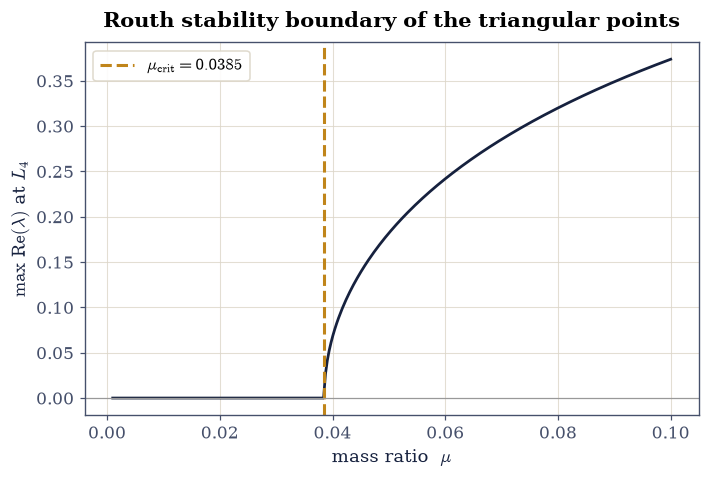
Fig. 162 Largest real part of the linear-stability eigenvalues at the triangular point \(L_4\) versus the mass ratio \(\mu\). It sits at zero (stable, purely oscillatory) until the Routh threshold \(\mu_{\rm crit}=\frac12(1-\sqrt{23/27})\approx0.0385\) (dashed), then lifts off positive (unstable). Below the line the Coriolis force traps a body at \(L_4\) despite \(\Omega\) being an unstable minimum there; above it, nothing can.

Validation 5

✓  the Routh critical mass ratio is ½(1−√(23/27)) ≈ 0.0385   [got 0.0385209 vs expected 0.0385209 (rtol=1e-09, atol=1e-09)]
✓  L4 is stable below μ_crit (Earth–Moon) and unstable above it (μ=0.06)   [Re(λ): μ=0.01215 → 1.07e-15,  μ=0.06 → 0.242]

True

Exercise 6 — Tadpole orbits near L4 (worked animation)

Now the payoff, and it genuinely moves. A test mass started just off \(L_4\), at rest in the rotating frame, does not fall into a primary and does not fly off: it librates around \(L_4\) on a long, curved tadpole orbit, the path swinging out toward \(L_3\) and back. This is exactly what Jupiter’s Trojan asteroids do at its \(L_4\) and \(L_5\). A still frame cannot convey the slow circulation, so we animate it.

Seeing it requires integrating the rotating-frame motion itself, which so far has only been differentiated, never advanced. As a first-order system in the state \(s = (x, y, \dot x, \dot y)\), Eq. 173 reads \(\dot s = (\dot x,\ \dot y,\ 2\dot y + \Omega_x,\ -2\dot x + \Omega_y)\): the gradient of \(\Omega\) drives the accelerations and the Coriolis terms \(\pm2\dot y, \mp2\dot x\) couple them. The validation confirms the mass stays bounded near \(L_4\) (a stable tadpole), the physics the animation shows.

Part a) Write rotating_rhs(t, s, mu), that state derivative, using the grad_Omega you built in Exercise 1 (the time argument is unused — solve_ivp requires it). Write this one yourself — the implementation is the lesson: this four-line right-hand side is the restricted three-body problem, and its equilibria are the five points located above.

Part b) Start a test mass at \(L_4 + (0.001, 0.001)\), at rest in the rotating frame, with \(\mu = 0.01215\). Using scipy.integrate.solve_ivp (its default RK45) with tolerances rtol=1e-10, atol=1e-12 and dense_output=True (sampled at 600 points), integrate from \(t = 0\) to \(t = 100\) and record the largest deviation from \(L_4\).

Part c) Animate the path, with the primaries and \(L_4\) marked.

max deviation from L4 over t∈[0,100] = 0.043  (bounded ⇒ tadpole)

Once Loop Reflect

Fig. 163 Animation of a test mass started just off \(L_4\) (at \(L_4+(0.001,0.001)\), at rest in the rotating frame, \(\mu=0.01215\)): instead of falling away it librates on a slow tadpole orbit around \(L_4\), swinging toward \(L_3\) and back. The primaries (grey) and \(L_4\) (amber) are fixed in this rotating frame. This is the motion of Jupiter’s Trojan asteroids; the validation confirms the orbit stays bounded near \(L_4\).

Validation 6

✓  the test mass stays bounded near L4: a stable tadpole orbit   [max deviation = 0.043 over t∈[0,100]]

True

Exercise 7 — The Jacobi constant and the unstable contrast (student exercise)

The rotating frame does work, so the test mass’s energy is not conserved. One combination is: the Jacobi constant Eq. 176, \(C = 2\Omega - v^2\). Checking that it stays flat along the tadpole orbit is an independent gate on the whole integration, and the contrast with an unstable point makes the stability concrete.

1. Write jacobi_constant(x, y, vx, vy, mu), the combination Eq. 176 \(C = 2\Omega - v^2\) with \(v^2 = \dot x^2 + \dot y^2\), from the Omega you built in Exercise 1. Write this one yourself — the implementation is the lesson: this one combination is the only integral of motion the restricted three-body problem has.

2. For the \(L_4\) orbit of Exercise 6, compute \(C(t)\) along the trajectory and confirm it is conserved even though the energy is not.

3. With scipy.integrate.solve_ivp (same rtol=1e-10, atol=1e-12) and the rotating_rhs you wrote in Exercise 6, integrate a test mass started at \(L_1 + (0.001, 0.001)\) (at rest, same \(\mu\)) to \(t = 20\) and show it diverges quickly, in contrast to the bounded \(L_4\) orbit.

4. Note what the conservation of \(C\) buys: the zero-velocity curve \(2\Omega = C\) bounds where the body can go.

Because the checks test the trajectory data (a conserved \(C\), a growing deviation), a ✗ points at the integration or the initial condition, not at any drawing.

Jacobi constant C ≈ 2.988003, relative drift = 1.15e-13

deviation near L1 after t=20: 0.27  (vs 0.043 near L4 over t=100)
zero-velocity fence: the orbit satisfies 2Ω >= C = 2.9880 throughout

Validation 7

✓  the Jacobi constant is conserved along the L4 trajectory   [max relative drift = 1.14886e-13 (limit 1e-06)]
✓  L1 is unstable (the test mass leaves its neighbourhood) while L4 stays bounded   [L1 deviation 0.27 (escapes) vs L4 deviation 0.043 (bounded)]

True

Exercise 8 — Where the Lagrange points live in the real solar system (synthesis)

The five points are not a textbook abstraction. The collinear \(L_2\) of the Sun–Earth system, \(1.5\) million km beyond the Earth, is where the James Webb Space Telescope parks: a single vantage with the Sun, Earth, and Moon all behind it. Because \(L_2\) is a saddle (Exercise 4), JWST does not sit at it but flies a halo orbit around it and burns a little fuel every few weeks to stay (station-keeping). The triangular points are different: stable, and so they collect material. At Jupiter’s \(L_4\) and \(L_5\) ride the Trojan asteroids, thousands of them, held for the age of the solar system because the Sun–Jupiter mass ratio sits far above the Routh threshold of 24.96. The same “equilibrium in an effective potential” idea reaches well beyond gravity, to the stationary points and saddles of molecular potential-energy surfaces and to many-body equilibria generally.

Jupiter carries a fraction \(\mu = 9.537\times10^{-4}\) of the Sun–Jupiter mass, and the Routh threshold of Eq. 175 reads \(m_1/m_2 > 24.96\) in mass-ratio form.

Part a) Confirm from those two numbers that the Sun–Jupiter pair clears the threshold, so its Trojan points are stable.

Sun–Jupiter mass ratio m1/m2 = 1047.5
Routh threshold              = 24.96  ⇒ Trojan points stable: True

Validation 8

✓  the Sun–Jupiter mass ratio exceeds 24.96, so the Trojan points are stable   [ratio = 1047.5]

True

Notebook summary

• The effective potential of the co-rotating frame, the collinear points \(L_1,L_2,L_3\) (roots of \(\partial\Omega/\partial x\) on the axis, by bracketed sign-change scan) and the triangular \(L_4,L_5\) shown to be exactly equilateral.

• Their stability: the collinear points are saddles; the triangular points are stable when the mass ratio clears the Routh threshold (\(\approx 0.0385\)). Tadpole orbits near \(L_4\), the Jacobi constant bounding the motion, and where the Lagrange points sit in the real solar system.

Outlook

• Halo and Lissajous orbits about the collinear points, and the station-keeping that JWST needs because \(L_2\) is unstable.

• Zero-velocity (Hill) curves from the Jacobi constant: the forbidden regions that open and close as \(C\) changes.

• Weak stability boundaries and low-energy transfers, the “interplanetary superhighway” that threads the collinear points’ invariant manifolds.

• Forward link. The effective-potential-equilibrium picture, stationary point plus Hessian stability, reappears for saddle points on molecular potential-energy surfaces, the same analysis in a different physical setting.

References

[MD99] (1,2,3)

Carl D. Murray and Stanley F. Dermott. Solar System Dynamics. Cambridge University Press, 1999.

[Nol16a]

Wolfgang Nolting. Theoretical Physics 1: Classical Mechanics. Springer, 2016. Grundkurs Theoretische Physik 1.

[Nol16b]

Wolfgang Nolting. Theoretical Physics 2: Analytical Mechanics. Springer, 2016.

[Sze67]

Victor Szebehely. Theory of Orbits: The Restricted Problem of Three Bodies. Academic Press, 1967.

Take this notebook with you

Use the download button (↓) in the toolbar above to save this notebook and run it yourself. The published notebooks ship without worked solutions; if you would like the reference solutions — to teach from or to check your own work — get in touch: hello@ramador.me.