6.15 Orbital Angular Momentum and the Spherical Harmonics

Elementary Computational Physics

Volume VI — Quantum Mechanics Notebook 6.15

The algebra, made into shapes. When angular momentum comes from actual motion in space, its operators become derivatives on the sphere and its eigenstates become the spherical harmonics — the same s, p, and d shapes that label every atomic orbital. The abstract spectrum of the previous notebook reappears as functions one can plot, and a single physical demand, that the wavefunction not contradict itself after a full turn, quietly forbids the half-integers and leaves them to spin.

Level · advanced   •   Est. · 160–195 min

Raymond Amador v1.4.0  ·  2026-07-31  ·  CC BY 4.0 (text) / MIT (code)

Notebook overview

The previous notebook (§6.14) built angular momentum from nothing but an algebra, and the spectrum fell out as abstract multiplets \(|j,m\rangle\) — vectors in a \((2j+1)\)-dimensional space, with no picture attached. This notebook gives the picture. When the angular momentum is orbital — when it comes from a particle actually moving through space, \(\mathbf{L}=\mathbf{r}\times\mathbf{p}\) — the operators stop being abstract matrices and become derivatives on the sphere, and their simultaneous eigenfunctions become concrete functions of the two angles: the spherical harmonics \(Y_l^m(\theta,\varphi)\).

Everything from §6.14 reappears, now realized in calculus. Writing \(\mathbf{p}=-i\hbar\nabla\) in spherical coordinates turns \(L_z\) into \(-i\hbar\,\partial/\partial\varphi\) and \(L^2\) into the angular part of the Laplacian — the radial coordinate drops out entirely, so angular momentum acts only on direction. The eigenvalue equations \(L^2Y_l^m=\hbar^2 l(l+1)Y_l^m\) and \(L_zY_l^m=\hbar m\,Y_l^m\) are the abstract \(j(j+1)\) and \(m\) spectra of §6.14, now satisfied by functions we can plot and integrate. The ladder operators \(L_\pm\) become differential operators that step between harmonics, and the spherical harmonics are orthonormal and complete on the sphere — the angular analogue of the Fourier basis (§6.9), the universal basis for any function of direction.

Then comes the twist the pure algebra could not see. The \(L_z\) eigenfunctions carry the factor \(e^{im\varphi}\), and a wavefunction in real space must be single-valued: advancing \(\varphi\) by \(2\pi\) returns to the same physical point, so \(e^{2\pi i m}=1\), which forces \(m\) — and hence \(l\) — to be an integer. The half-integers that the algebra of §6.14 permitted have no orbital realization. They survive only for spin, which has no position-space wavefunction and so escapes the argument entirely. This is the deep reason spin is called “intrinsic”: the algebra permits half-integers, geometry forbids them for orbital motion, and spin is precisely what is left over.

Finally we connect to chemistry. The complex \(Y_l^m\) are the \(L_z\) eigenstates; their real combinations are the familiar orbital shapes — \(s\) (spherical), \(p\) (two lobes), \(d\) (cloverleaves) — the real spherical harmonics first built in Volume III, reused here. Every atomic orbital ever drawn is one of these functions, and they had to be these and no others, because the algebra of rotation and the geometry of the sphere left no other choice.

As in every Volume VI notebook, each exercise opens with a crystal-clear statement and enumerated parts, each naming the exact operation — scipy.special.sph_harm_y for the harmonics, the angular Laplacian by finite differences in \(\theta\) and the periodic \(\varphi\), and numpy.trapezoid with the \(\sin\theta\) measure for inner products on the sphere.

Conventions and method notes. \(\hbar=1\). We use the current SciPy API scipy.special.sph_harm_y(n, m, theta, phi) with \(n=l\) the degree, \(\theta\in[0,\pi]\) the polar (colatitude) angle, and \(\varphi\in[0,2\pi)\) the azimuth — note the old scipy.special.sph_harm was removed, and both its name and its argument order (\(\mathrm{sph\_harm}(m,l,\varphi,\theta)\)) have changed. The operators \(L_z,L^2,L_\pm\) are realized as finite differences on a \((\theta,\varphi)\) grid; the \(1/\sin\theta\) factors in \(L^2\) and \(L_\pm\) make the finite differences degrade near the poles, so we verify eigenvalue equations in the bulk (\(\theta\) away from \(0,\pi\)) and say so. \(L_z=-i\hbar\,\partial_\varphi\) has no such factor and is reliable everywhere. See Sakurai & Napolitano (§3.6); Griffiths (the angular equation); and Notebooks §6.14 (the algebra/spectrum/ladder, here realized), §6.6 (incompatibility), §6.9 (the basis-expansion idea), and Volume III (the real spherical harmonics and orbital visualization).

Theory in brief

Orbital angular momentum as a differential operator

For a particle moving in space, \(\mathbf{L}=\mathbf{r}\times\mathbf{p}\) with \(\mathbf{p}=-i\hbar\nabla\). In spherical coordinates this becomes purely angular,

(572)\[L_z=-i\hbar\,\frac{\partial}{\partial\varphi},\qquad L^2=-\hbar^2\left[\frac{1}{\sin\theta}\frac{\partial}{\partial\theta}\Big(\sin\theta\,\frac{\partial}{\partial\theta}\Big)+\frac{1}{\sin^2\theta}\frac{\partial^2}{\partial\varphi^2}\right],\]

exactly the angular part of the Laplacian \(\nabla^2\). The radial coordinate has dropped out: angular momentum acts only on direction. These operators satisfy the same algebra \([L_i,L_j]=i\hbar\, \varepsilon_{ijk}L_k\) as §6.14, now realized in calculus.

The spherical harmonics

The simultaneous eigenfunctions of \(L^2\) and \(L_z\) are the spherical harmonics,

(573)\[L^2 Y_l^m=\hbar^2 l(l+1)\,Y_l^m,\qquad L_z Y_l^m=\hbar m\,Y_l^m,\qquad Y_l^m(\theta,\varphi)=N_{lm}\,P_l^m(\cos\theta)\,e^{im\varphi},\]

where \(e^{im\varphi}\) carries the \(L_z\) eigenvalue and the associated Legendre function \(P_l^m(\cos\theta)\) gives the polar shape. These are the abstract \(|j,m\rangle\to|l,m\rangle\) multiplets of §6.14, now functions on the sphere.

Orthonormality and completeness

Under the inner product with the spherical area measure \(\sin\theta\,d\theta\,d\varphi\),

(574)\[\langle Y_l^m\,|\,Y_{l'}^{m'}\rangle=\int_0^{2\pi}\!\!\int_0^\pi Y_l^{m\,*}\,Y_{l'}^{m'}\,\sin\theta\,d\theta\,d\varphi=\delta_{ll'}\delta_{mm'},\]

the spherical harmonics are orthonormal, and they are complete: any function on the sphere expands as \(\sum_{l,m}c_{lm}Y_l^m\) (the angular analogue of the basis expansions of §6.1 and §6.9). This is why they are the universal angular basis.

The ladder operators on the sphere

The raising and lowering operators \(L_\pm=L_x\pm iL_y\) become

(575)\[L_\pm=\hbar\,e^{\pm i\varphi}\Big(\pm\frac{\partial}{\partial\theta}+i\cot\theta\,\frac{\partial}{\partial\varphi}\Big),\qquad L_\pm Y_l^m=\hbar\sqrt{l(l+1)-m(m\pm1)}\;Y_l^{m\pm1},\]

the abstract ladder of §6.14, now a differential operator stepping between spherical harmonics — \(L_+\) annihilates the top \(Y_l^{\,l}\) and \(L_-\) the bottom \(Y_l^{-l}\).

Why \(l\) and \(m\) are integers

The \(L_z\) eigenfunctions carry \(e^{im\varphi}\). Physical single-valuedness — the wavefunction must return to itself when \(\varphi\) advances by \(2\pi\) — demands

(576)\[e^{im(\varphi+2\pi)}=e^{im\varphi}\ \Longrightarrow\ e^{2\pi i m}=1\ \Longrightarrow\ m\in\mathbb{Z},\]

and the ladder then forces \(l\in\{0,1,2,\dots\}\). So orbital angular momentum admits only integer values: the half-integers the pure algebra allowed (§6.14) are excluded for orbital motion. They survive only for spin, which has no position-space wavefunction and escapes the single-valuedness argument — the deep reason spin is “intrinsic.”

The orbital shapes

The complex \(Y_l^m\) are \(L_z\) eigenstates; the real linear combinations \(Y_l^m\pm Y_l^{-m}\) are the familiar orbital shapes,

(577)\[l=0\ (s,\ \text{spherical}),\quad l=1\ (p,\ \text{two lobes}),\quad l=2\ (d,\ \text{cloverleaves}),\ \dots\qquad 2l+1\ \text{orbitals per shell},\]

the real spherical harmonics of Volume III, reused here. The labels \(l=0,1,2,3\) are \(s,p,d,f\); the count \(2l+1\) is the number of \(m\) values. This is the angular skeleton of the periodic table.

Setup

The data are the series palette, the convention \(\hbar=1\), and the spherical harmonics themselves, which arrive ready-made from scipy.special.sph_harm_y — this notebook studies them, it does not construct them. The instruments are the \((\theta,\varphi)\) grid the operators are discretized on with its polar “bulk” mask, the bulk-ratio reader that turns an applied operator into an eigenvalue, and the real spherical harmonics, built from scratch in §3.5 and restated here as a tool. The operators themselves are deliberately absent: you build \(L_z\) in Exercise 1, \(L^2\) in Exercise 2, the spherical inner product in Exercise 3, and \(L_+\) in Exercise 4.

The Setup below holds this notebook’s data and instruments — nothing you are asked to build. It is collapsed so the building stays yours; expand it whenever you want the details.

Show code cell source

Hide code cell source

import matplotlib.pyplot as plt
import numpy as np
from scipy.special import sph_harm_y

from ecp import draw, validate

# data: the series palette
ACCENT, INK = draw.ACCENT, draw.INK
RED, BLUE = "#c1121f", "#1d4e89"

HBAR = 1.0

# instrument: the (theta, phi) grid the operators are sampled on — theta polar in [0, pi], phi
# azimuth in [0, 2pi) (periodic). A discretization choice, not the lesson: the operators you build
# in Exercises 1, 2 and 4 read their spacings (DTH, DPH) and their trigonometry (SIN_TH, TH, PH)
# from here.
N_THETA, N_PHI = 300, 300
THETA = np.linspace(0.0, np.pi, N_THETA)
PHI = np.linspace(0.0, 2 * np.pi, N_PHI, endpoint=False)
DTH = THETA[1] - THETA[0]
DPH = PHI[1] - PHI[0]
TH, PH = np.meshgrid(THETA, PHI, indexing="ij")
SIN_TH = np.sin(TH)
# the "bulk" excludes a margin around the poles, where the 1/sinθ finite differences degrade
BULK = (TH > 0.20) & (TH < np.pi - 0.20)


# data: the specimen this notebook studies. The harmonics arrive ready-made from
# scipy.special.sph_harm_y — there is nothing here to construct, and the wrapper exists only to
# pin the current SciPy signature. What you build are the operators they are eigenfunctions of.
def spherical_harmonic(l, m, theta, phi):
    """The spherical harmonic $Y_l^m(\\theta,\\varphi)$, via ``scipy.special.sph_harm_y``.

    Uses the **current** SciPy signature ``sph_harm_y(n=l, m, theta, phi)`` with $\\theta\\in[0,\\pi]$ the
    polar angle and $\\varphi\\in[0,2\\pi)$ the azimuth. (The old ``scipy.special.sph_harm`` was removed;
    both its name and its argument order — ``sph_harm(m, l, phi, theta)`` — changed.) The structure is
    $Y_l^m=N_{lm}P_l^m(\\cos\\theta)e^{im\\varphi}$ {eq}`eq-orbital-spherical-harmonics`.
    """
    return sph_harm_y(l, m, theta, phi)


# instrument: a reading device. It converts an already-applied operator into a number by taking
# the median ratio over the poles-excluded grid where the amplitude is not tiny — numerical
# hygiene against polar finite-difference error and division by near-zero, not the operator
# physics it is used to check.
def eigenvalue_in_bulk(L_field, field):
    """Read the eigenvalue of a (numerically applied) operator as the bulk ratio ``L_field / field``.

    Takes the median of $L_\\text{field}/\\text{field}$ over the bulk grid where $|\\text{field}|$ is not
    tiny, avoiding both the polar finite-difference error and division by near-zero amplitudes.
    """
    mask = BULK & (np.abs(field) > 0.05 * np.abs(field).max())
    return np.median((L_field[mask] / field[mask]).real)


# built from scratch in §3.5 (Exercise 6, where the cosine/sine combinations are assembled and
# drawn as the orbital lobes); restated here as an instrument.
def real_spherical_harmonic(l, m, theta, phi):
    """The **real** spherical harmonic (the orbital shape), built from ``sph_harm_y`` (Volume III).

    The familiar chemist's orbitals: $Y_l^0$ real for $m=0$, and for $m\\ne0$ the real/imaginary
    combinations $Y_l^{m,\\text{real}}\\propto P_l^{|m|}\\cos|m|\\varphi$ (or $\\sin|m|\\varphi$) that carry
    the azimuthal lobes. These are the $s,p,d,f$ shapes {eq}`eq-orbital-shapes`, reused from Volume III's
    multipole-expansion notebook.
    """
    if m == 0:
        return sph_harm_y(l, 0, theta, phi).real
    if m > 0:
        return np.sqrt(2.0) * (-1.0) ** m * sph_harm_y(l, m, theta, phi).real
    return np.sqrt(2.0) * (-1.0) ** m * sph_harm_y(l, -m, theta, phi).imag

Exercise 1 — \(L_z\) as a differential operator

For orbital motion the abstract \(J_z\) of §6.14 stops being a matrix and becomes a derivative in the azimuthal angle, \(L_z=-i\hbar\,\partial/\partial\varphi\) Eq. 572 — the algebra realized in calculus. Its eigenfunctions are the spherical harmonics, with eigenvalue \(\hbar m\) Eq. 573, and it is the factor \(e^{im\varphi}\) in \(Y_l^m\) that carries that eigenvalue: differentiating it in \(\varphi\) brings down \(im\), which is the whole reason \(L_z\) is nothing more than \(-i\hbar\,\partial_\varphi\). On a grid the azimuth is periodic, so the \(\varphi\)-derivative is a central difference that wraps around \(\varphi=2\pi\) (numpy.roll along the azimuth axis). Unlike the operators that follow, \(L_z\) carries no \(1/\sin\theta\) factor, so it is accurate everywhere on the sphere, poles included.

1. Write Lz_operator(field), applying \(L_z=-i\hbar\,\partial_\varphi\) to a field on the \((\theta,\varphi)\) grid as a periodic central difference in \(\varphi\) (spacing DPH). Write this one yourself — the implementation is the lesson.

2. Build \(Y_l^m\) on the grid with spherical_harmonic (which wraps scipy.special.sph_harm_y(l, m, theta, phi)).

3. Apply your \(L_z\) to it.

4. Confirm the result is \(\hbar m \,Y_l^m\) by reading the bulk ratio with eigenvalue_in_bulk.

Lz Yₗᵐ = ℏm Yₗᵐ  (finite-difference ∂_φ, ℏ=1):
  l=1, m=+1:  Lz Yₗᵐ / Yₗᵐ = +0.99993   (expected m = +1)
  l=2, m=-1:  Lz Yₗᵐ / Yₗᵐ = -0.99993   (expected m = -1)
  l=2, m=+2:  Lz Yₗᵐ / Yₗᵐ = +1.99942   (expected m = +2)
  l=3, m=+2:  Lz Yₗᵐ / Yₗᵐ = +1.99942   (expected m = +2)

the e^{imφ} factor carries the Lz eigenvalue — Lz is just −iℏ∂/∂φ

Validation 1

✓  the spherical harmonics are Lz eigenfunctions with eigenvalue ℏm (Lz = −iℏ∂/∂φ, finite difference)

True

Exercise 2 — \(L^2\) as the angular Laplacian

The second operator is the angular part of the Laplacian, \(L^2=-\hbar^2[(1/\sin\theta) \partial_\theta(\sin\theta\,\partial_\theta)+(1/\sin^2\theta)\partial_\varphi^2]\) Eq. 572, and the spherical harmonics are its eigenfunctions with eigenvalue \(\hbar^2 l(l+1)\) Eq. 573 — the same \(j(j+1)\) the algebra of §6.14 produced, now an eigenvalue of a derivative operator: the algebraic spectrum as calculus. Discretizing it needs two different stencils, because the two angles are not alike: numpy.gradient in \(\theta\), which is not periodic, and a periodic central second difference in \(\varphi\). Note also that the \(\theta\) term is not a plain second derivative — the \(\sin\theta\) sits between the two \(\theta\)-derivatives and must be applied there. The \(1/\sin\theta\) prefactors blow up at \(\theta=0,\pi\), so the eigenvalue is read in the bulk, away from the poles, with a looser tolerance than \(L_z\) needed.

1. Write L2_operator(field), applying \(L^2\) to a field on the \((\theta,\varphi)\) grid by those finite differences. Write this one yourself — the implementation is the lesson.

2. Apply it to \(Y_l^m\).

3. Confirm the eigenvalue is \(\hbar^2 l(l+1)\) in the bulk with eigenvalue_in_bulk.

L² Yₗᵐ = ℏ²l(l+1) Yₗᵐ  (angular Laplacian, bulk away from poles):
  l=1, m=+0:  L² Yₗᵐ / Yₗᵐ =  1.9998   (expected l(l+1) = 2)
  l=2, m=+0:  L² Yₗᵐ / Yₗᵐ =  5.9984   (expected l(l+1) = 6)
  l=2, m=+1:  L² Yₗᵐ / Yₗᵐ =  5.9990   (expected l(l+1) = 6)
  l=3, m=+2:  L² Yₗᵐ / Yₗᵐ = 11.9975   (expected l(l+1) = 12)

the same l(l+1) spectrum the algebra gave in §6.14 — now a differential-operator eigenvalue

Validation 2

✓  the spherical harmonics are L² eigenfunctions with eigenvalue ℏ²l(l+1) (the §6.14 spectrum realized as the angular Laplacian, verified in the bulk)

True

Exercise 3 — Orthonormality on the sphere

What makes a set of functions a basis is the inner product it is orthonormal under, and on the sphere that inner product carries the area measure \(\sin\theta\,d\theta\,d\varphi\): \(\langle Y|Y'\rangle=\int Y^*Y'\sin\theta\,d\theta\,d\varphi\), under which \(\langle Y_l^m|Y_{l'}^{m'} \rangle=\delta_{ll'}\delta_{mm'}\) Eq. 574. On the grid the two angles again want different treatment: numpy.trapezoid in \(\theta\), where the endpoints \(0,\pi\) are real edges, and in the periodic azimuth a plain sum \(\times\,d\varphi\), which needs no end correction because the last sample’s neighbour is the first. Orthonormality is half the story; the harmonics are also complete, so any function on the sphere expands as \(\sum_{l,m}c_{lm}Y_l^m\) — the universal angular basis, the basis idea of §6.1/§6.9 now on the sphere.

1. Write sphere_inner(Y1, Y2), the spherical inner product \(\int Y_1^*Y_2\,\sin\theta\,d\theta \,d\varphi\) evaluated on the \((\theta,\varphi)\) grid with the \(\sin\theta\) measure.

2. Compute \(\langle Y_l^m|Y_l^m\rangle=1\) for several \((l,m)\) (normalization).

3. Compute \(\langle Y_l^m|Y_{l'}^{m'} \rangle=0\) for different \((l,m)\) (orthogonality).

  ⟨Y_0^+0 | Y_0^+0⟩ = 0.999991
  ⟨Y_1^+1 | Y_1^+1⟩ = 1.000000
  ⟨Y_2^+0 | Y_2^+0⟩ = 0.999954
  ⟨Y_2^-1 | Y_2^-1⟩ = 1.000000
  ⟨Y_3^+2 | Y_3^+2⟩ = 1.000000

  |⟨Y_1^+0 | Y_2^+0⟩| = 2.78e-17
  |⟨Y_2^+1 | Y_2^-1⟩| = 1.19e-16
  |⟨Y_1^+1 | Y_3^+1⟩| = 5.70e-10

orthonormal and complete: any angular function expands as Σ cₗₘ Yₗᵐ (the sphere's Fourier basis)

Validation 3

✓  the spherical harmonics are orthonormal on the sphere under the sinθ measure   [max|Δ| = 4.60004e-05 (rtol=1e-06, atol=0.01)]

True

Exercise 4 — The ladder on the sphere

The ladder of §6.14 survives the translation into calculus as a differential operator stepping between functions: \(L_\pm=\hbar\,e^{\pm i\varphi}(\pm\partial_\theta+i\cot\theta\,\partial_\varphi)\), with \(L_+Y_l^m=\hbar\sqrt{l(l+1)-m(m+1)}\,Y_l^{m+1}\) Eq. 575. Starting from \(m=0\) the coefficient is \(\hbar\sqrt{l(l+1)-0}=\hbar\sqrt{l(l+1)}\), and on the top rung \(m=l\) it vanishes, so \(L_+Y_l^{\,l}=0\) — the ladder terminates, exactly as the algebra said it must. The \(\cot\theta\) carries the same polar disease as the \(1/\sin\theta\) of \(L^2\), so both facts are read in the bulk.

1. Write Lplus_operator(field), applying \(L_+=\hbar e^{i\varphi}(\partial_\theta+i\cot\theta\, \partial_\varphi)\) to a field on the \((\theta,\varphi)\) grid. Write this one yourself — the implementation is the lesson.

2. Apply it to \(Y_l^0\).

3. Confirm the result is proportional to \(Y_l^1\) with coefficient \(\hbar\sqrt{l(l+1)}\) (the bulk ratio against \(Y_l^1\)).

4. Confirm \(L_+\) annihilates the top rung \(Y_l^{\,l}\) (its bulk norm is negligible).

L₊ Yₗ⁰ = ℏ√(l(l+1)) Yₗ¹  (the ladder as a differential operator):

  l=1:  L₊Yₗ⁰ / Yₗ¹ = 1.4142   (expected √(l(l+1)) = 1.4142)
  l=2:  L₊Yₗ⁰ / Yₗ¹ = 2.4493   (expected √(l(l+1)) = 2.4495)
  l=3:  L₊Yₗ⁰ / Yₗ¹ = 3.4636   (expected √(l(l+1)) = 3.4641)

L₊ annihilates the top rung Yₗˡ (the ladder terminates):
  l=1:  ‖L₊ Yₗˡ‖ / ‖Yₗˡ‖ (bulk) = 0.0000

  l=2:  ‖L₊ Yₗˡ‖ / ‖Yₗˡ‖ (bulk) = 0.0003

Validation 4

✓  L₊ raises m with coefficient ℏ√(l(l+1)−m(m+1)) and annihilates the top rung Yₗˡ — the §6.14 ladder as a differential operator

True

Exercise 5 — Why \(l\) and \(m\) are integers

The \(L_z\) eigenfunctions carry the factor \(e^{im\varphi}\), and a wavefunction in real space must be single-valued: advancing \(\varphi\) by a full turn returns to the same physical point, so \(e^{im(\varphi+2\pi)}=e^{im\varphi}\), that is \(e^{2\pi im}=1\) Eq. 576. This is a constraint the pure algebra of §6.14 could not see, and it is what excludes the half-integer angular momenta that the algebra permitted.

1. Confirm with numpy.exp that \(e^{2\pi im}=1\) holds only for integer \(m\) (test \(m=\tfrac12,1,\tfrac32,2,\tfrac52\)).

2. Conclude orbital angular momentum has only integer \(l\); the half-integers belong to spin, which has no position-space wavefunction and so escapes the argument. The algebra permits half-integers, geometry forbids them for orbital motion, and spin is what remains.

single-valuedness e^{2πim} = 1 ?
  m = 0.5:  e^(2πim) = -1.000+0.000j   |e^(2πim) − 1| = 2.000   DOUBLE-VALUED (sign flips after 2π — rejected)
  m = 1.0:  e^(2πim) = +1.000-0.000j   |e^(2πim) − 1| = 0.000   single-valued (allowed)
  m = 1.5:  e^(2πim) = -1.000+0.000j   |e^(2πim) − 1| = 2.000   DOUBLE-VALUED (sign flips after 2π — rejected)
  m = 2.0:  e^(2πim) = +1.000-0.000j   |e^(2πim) − 1| = 0.000   single-valued (allowed)
  m = 2.5:  e^(2πim) = -1.000+0.000j   |e^(2πim) − 1| = 2.000   DOUBLE-VALUED (sign flips after 2π — rejected)

only INTEGER m survive: orbital angular momentum is integer-only (l = 0,1,2,…)
the half-integers of §6.14 belong to SPIN — which has no position-space wavefunction to be single-valued

Validation 5

✓  single-valuedness (e^{2πim}=1) holds only for integer m, so orbital l,m are integers — the half-integers of §6.14 are excluded and belong to spin

True

Exercise 6 — The orbital shapes: from \(Y_l^m\) to \(s,p,d\)

The complex \(Y_l^m\) are \(L_z\) eigenstates, but chemistry draws their real combinations \(Y_l^m\pm Y_l^{-m}\): the familiar orbital shapes — \(s\) (spherical), \(p\) (lobed), \(d\) (cloverleaves) — with \(2l+1\) of them per shell Eq. 577. They are the real spherical harmonics built in §3.5 and restated in the Setup here. The labels \(s,p,d,f\) are nothing but \(l=0,1,2,3\), and the count \(2l+1\) is the number of \(m\) values: the \(L^2,L_z\) eigenfunctions are the orbitals of chemistry, and the spherical harmonics are the angular skeleton of the periodic table.

1. Form the real combinations with the real_spherical_harmonic helper.

2. Check the structural facts: \(s\) (\(l=0\)) is constant in angle (spherical), \(p_z\) (\(l=1,m=0\)) is \(\propto\cos\theta\) (sign-flips across the equator), and there are \(2l+1\) functions for each \(l\).

3. Plot the \(s,p,d\) real orbitals as 3-D surfaces (radius \(\propto|Y^{\text{real}}|\), color by sign).

s (l=0) is spherical (constant in angle): True  [value 0.2821 = 1/√4π]
p_z (l=1,m=0) ∝ cosθ, sign flips across the equator: True
   ⟨p_z⟩ north = +0.332,  south = -0.332
there are 2l+1 orbitals per shell (l=0..3 → [1, 3, 5, 7]): True
labels: l = 0,1,2,3 → s,p,d,f — the angular skeleton of the periodic table

Validation 6

✓  the real spherical harmonics are the s/p/d orbital shapes (s spherical, p_z lobed with a sign change, 2l+1 per shell) — the atomic orbitals (Volume III)

True

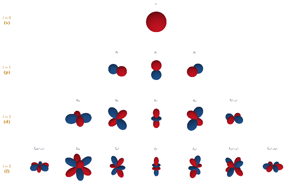
Fig. 550 The spherical harmonics are the atomic orbitals — the full \(s,p,d,f\) gallery. Three-dimensional surfaces of the real spherical harmonics (scipy.special.sph_harm_y, the Volume III construction), one row per shell \(l=0,1,2,3\): the radius is \(\propto|Y_{lm}^{\text{real}}|\) and the color is its sign (red positive, blue negative). Each shell holds exactly \(2l+1\) orbitals — the \(l=0\) \(s\) (one featureless sphere), the three \(l=1\) \(p\) dumbbells along \(x,y,z\), the five \(l=2\) \(d\) shapes (four cloverleaves and the \(d_{z^2}\) with its polar lobes and equatorial collar), and the seven \(l=3\) \(f\) shapes. The number of angular nodes grows with \(l\): reading a shape, the count of polar nodal circles is \(l-|m|\) and the azimuthal lobing is set by \(|m|\), so the higher shells are progressively more structured. These are exactly the \(s,p,d,f\) shapes drawn in every chemistry text, and they are nothing more than the simultaneous eigenfunctions of \(L^2\) and \(L_z\) — forced to be these and no others by the algebra of rotation and the geometry of the sphere.

The phase behind the shapes

The gallery above is deceptively still. Each surface is the modulus \(|Y_l^m|\), but \(Y_l^m\) is a complex wave, and the lobe pictures quietly throw away its phase \(e^{im\varphi}\). Worse, a stationary state is not actually frozen: it evolves in time as \(\psi(t)=Y_l^m\,e^{-iEt/\hbar}\) (the time-evolution of §6.7). Because \(e^{-iEt/\hbar}\) is a global phase, the probability density \(|\psi(t)|^2=|Y_l^m|^2\) stands perfectly still — nothing observable changes — yet the phase itself keeps turning underneath.

Colouring each fixed lobe by its running phase \(\arg(Y_l^m e^{-iEt})\) makes that hidden turning visible, and with it the physical meaning of the quantum number \(m\). For \(m\ne0\) the colour circulates around the \(z\)-axis, winding \(m\) times: a running wave that carries angular momentum \(\hbar m\) about \(z\) — this is what “magnetic quantum number” means. For \(m=0\) the real harmonic simply pulses in place, a standing wave with no azimuthal current. The illustration below (not an exercise) animates one full period; watch the colour circulate for \(m\ne0\) and pulse for \(m=0\), while every shape holds still.

Once Loop Reflect

Fig. 551 Colour is phase: a stationary state is a standing wave whose phase turns. Each surface is a fixed orbital lobe \(|Y_l^m|\), coloured by its running phase \(\arg(Y_l^m e^{-iEt})\) on a cyclic colormap (Matplotlib’s twilight), stepped through one full period \(T=2\pi/E\). The shapes never move, and the probability density \(|\psi|^2=|Y_l^m|^2\) is exactly constant in time (drift \(\sim10^{-16}\)) — what turns is the phase, not the electron. For \(m\ne0\) the colour circulates about the \(z\)-axis, winding \(m\) times (\(Y_1^1\) once, \(Y_2^2\) twice, \(Y_3^3\) thrice) and rotating rigidly: this running wave is the angular momentum \(\hbar m\) about \(z\), the physical meaning of the magnetic quantum number. For \(m=0\) (\(Y_1^0\)) the harmonic is real, so the colour merely pulses in place — a standing wave carrying no azimuthal current. The animation shows the wave, not the motion of a particle: this is a stationary state, and nothing observable about it changes with time.

With your assistant

The gallery machinery of Exercise 6 — meshgrids, 3-D axes, colormaps, view angles — is visualization plumbing, and delegating it outright is exactly what the plumbing deserves. The physics cells stay yours: whatever your assistant renders, confirm the surfaces it drew are \(|Y_l^m|\) on the correct \((\theta,\phi)\) grid by checking one value you can compute by hand — \(|Y_0^0| = 1/\sqrt{4\pi}\) everywhere is enough to catch a swapped axis. The check is yours.

Exercise 7 — A superposition on the sphere and its angular-momentum statistics (student)

An angular wavefunction need not be a single harmonic. Expanded in the basis, \(\psi(\theta,\varphi)=\sum c_{lm}Y_l^m\), it is the postulates of Movement I applied to angular momentum: the Born rule (§6.5) in the angular basis makes \(|c_{lm}|^2\) the probability of measuring \((l,m)\), and because the harmonics are orthonormal Eq. 573, Eq. 574 the normalization is simply \(\langle\psi|\psi\rangle=\sum|c_{lm}|^2\). The expectation values then follow from the eigenvalues alone, \(\langle L_z\rangle=\sum|c_{lm}|^2\hbar m\) and \(\langle L^2\rangle=\sum|c_{lm}|^2\hbar^2 l(l+1)\) — and \(\langle L_z\rangle\) can be had a second way, as the operator expectation \(\langle\psi|L_z|\psi\rangle\), which is worth doing because \(L_z\) is the pole-free operator and can therefore be integrated over the full sphere.

1. Build \(\psi(\theta,\varphi)=\sum c_{lm}Y_l^m\) with given coefficients and normalize it with the sphere_inner you wrote in Exercise 3.

2. Read off the probability of measuring \((l,m)\) as \(|c_{lm}|^2\).

3. Compute \(\langle L_z\rangle\) and \(\langle L^2\rangle\) from those probabilities.

4. Verify \(\langle L_z\rangle\) directly as \(\langle\psi|L_z|\psi\rangle\), with your Exercise 1 Lz_operator and the full-sphere inner product.

measurement probabilities |cₗₘ|² (Born rule on the sphere):
   P(l=1, m=+0) = 0.3600
   P(l=2, m=+1) = 0.4096
   P(l=2, m=-1) = 0.2304
   Σ P = 1.0000

⟨Lz⟩ from |cₗₘ|²:  +0.17920
⟨Lz⟩ from the operator ⟨ψ|Lz|ψ⟩:  +0.17919   (agree)
⟨L²⟩ from |cₗₘ|²:  4.56005   (each Yₗᵐ is an L² eigenfunction, Exercise 2)

Validation 7

✓  the Born rule on the sphere: the probabilities |cₗₘ|² sum to 1 and ⟨Lz⟩=Σ|cₗₘ|²ℏm matches the direct operator expectation ⟨ψ|Lz|ψ⟩

True

Exercise 8 — The shapes of angular momentum (synthesis)

When angular momentum comes from real motion through space, the operators we built abstractly in §6.14 become derivatives on the sphere, and their eigenstates become the spherical harmonics — the very \(s\), \(p\), and \(d\) shapes that organize the periodic table. The abstract spectrum \(\hbar^2 l(l+1)\), \(\hbar m\) reappeared as functions we could plot and integrate; the ladder became a differential operator stepping between them; and a single physical demand — that a wavefunction not contradict itself after a full turn — quietly excluded the half-integers, handing them to spin.

There is no new computation here: the realization is the result. The half-integers of §6.14 were not wrong; they were simply not orbital. Single-valuedness on the sphere is a constraint the pure algebra could not feel, and it is exactly what separates the integer orbital angular momenta — which have a position-space wavefunction \(Y_l^m(\theta,\varphi)\) — from the half-integer spins, which do not. With the angular problem now solved once and for all, the next notebook (§6.16) attacks the full three-dimensional Schrödinger equation: separate the angular part (these spherical harmonics) from the radial part, and any central-force problem collapses to a one-dimensional radial equation of the kind we already solved in §6.10–§6.11. That is the road to hydrogen (§6.17).

Every atomic orbital you have ever seen drawn is one of these functions. The chemist’s \(s\), \(p\), and \(d\) are not mnemonics — they are the eigenfunctions of \(L^2\) and \(L_z\), and they had to be these and nothing else, because the algebra of rotation and the geometry of the sphere left no other choice.

Notebook summary

The algebra of §6.14, realized as calculus on the sphere — the second notebook of Movement III.

• Orbital operators Eq. 572: \(L_z=-i\hbar\,\partial_\varphi\) and \(L^2\) the angular Laplacian — the radial coordinate drops out, so angular momentum acts only on direction.

• The spherical harmonics Eq. 573: \(L^2Y_l^m=\hbar^2 l(l+1)Y_l^m\), \(L_zY_l^m= \hbar m Y_l^m\) (verified on a grid via scipy.special.sph_harm_y) — the §6.14 spectrum as functions.

• Orthonormality Eq. 574: \(\langle Y_l^m|Y_{l'}^{m'}\rangle=\delta_{ll'} \delta_{mm'}\) under the \(\sin\theta\) measure — the universal, complete angular basis (§6.1/§6.9).

• The ladder Eq. 575: \(L_\pm\) as differential operators stepping between harmonics, with coefficient \(\hbar\sqrt{l(l+1)-m(m\pm1)}\), annihilating the top/bottom rung.

• Integers only Eq. 576: single-valuedness \(e^{2\pi im}=1\) forces \(l,m\in \mathbb{Z}\) — the half-integers of §6.14 are excluded for orbital motion and belong to spin.

• The orbital shapes Eq. 577: the real \(Y_l^m\) are the \(s,p,d,f\) orbitals, \(2l+1\) per shell (Volume III) — the angular skeleton of the periodic table.

The abstract multiplets became plottable functions, and geometry quietly forbade the half-integers. The angular problem is solved; the radial problem is next.

Outlook

• The three-dimensional Schrödinger equation (§6.16): separation of variables — the angular part is solved (these spherical harmonics), the radial part becomes a 1-D equation of the §6.10–§6.11 kind.

• The hydrogen atom (§6.17): the Coulomb radial equation meeting these angular solutions — the crown jewel of the volume.

• Spin (§6.18) and the addition of angular momenta (§6.19): the half-integers excluded here, and their coupling to orbital motion.

• Selection rules and the shapes of spectral lines (a horizon; time-dependent transitions, §6.24).

• Cross-reference §6.14 (the algebra, spectrum, and ladder, here realized), §6.6 (incompatibility), §6.5 (the Born rule), Volume III (the real spherical harmonics), and forward to §6.16, §6.17, §6.18.

Take this notebook with you

Use the download button (↓) in the toolbar above to save this notebook and run it yourself. The published notebooks ship without worked solutions; if you would like the reference solutions — to teach from or to check your own work — get in touch: hello@ramador.me.