


4.7 The Relativistic Lagrangian and Motion in Fields#
Notebook overview#
This notebook is where two long threads of the course tie together. Volume II made mechanics variational — motion extremizes an action — and Volume III built electrodynamics, culminating in the field tensor \(F^{\mu\nu}\) of §3.12 that fused \(\mathbf E\) and \(\mathbf B\) into one object. Here both become relativistic and meet. The free relativistic particle turns out to extremize its proper time, so the fact of §4.4 that the inertial worldline is the longest becomes a genuine variational principle; and a charge in a field moves under the covariant Lorentz force \(dp^\mu/d\tau=qF^{\mu\nu}u_\nu\), the tensor of §3.12 now driving dynamics. This is the explicit Volume III \(\leftrightarrow\) Volume IV handshake.
From the single Lagrangian \(L=-mc^2\sqrt{1-v^2/c^2}\) we recover the canonical momentum \(\gamma m\mathbf v\) and energy \(\gamma mc^2\) of §4.5 — now from a variational principle rather than a postulate — and, with Noether’s theorem from §2.2, the conservation of four-momentum. Adding the electromagnetic coupling gives the equation of motion, whose covariant form we verify reproduces the familiar \(q(\mathbf E+\mathbf v\times\mathbf B)\) by contracting the field tensor of §3.12 with the four-velocity. We then put a real particle in real fields and integrate its trajectory: the relativistic cyclotron, whose frequency \(\omega=qB/(\gamma m)\) falls with energy (the flaw that forced the invention of the synchrotron), and the \(\mathbf E\times\mathbf B\) drift of crossed fields, a building block of plasma physics.
We reuse the four-vector and np.einsum machinery of §4.3 and §4.5 and the field tensor of
§3.12 by cross-reference, not rederivation. Trajectories are integrated with
scipy.integrate.solve_ivp (DOP853), with the relativistic subtlety handled by carrying the
momentum as the state variable and recovering the velocity from it, so the
\(\gamma\)-dependence never needs inverting by hand. One trajectory, the cyclotron orbit, is
genuine motion and is animated; the rest are clean stills.
Everything is in SI units, with \(c=1/\sqrt{\mu_0\varepsilon_0}=2.998\times10^8\,\)m/s and stated charges, masses, fields, and initial conditions.
How to read the checks. Each exercise closes with a
validatecall against an independent fact: the canonical momentum \(\gamma mv\); the covariant force equal to \(q(\mathbf E+\mathbf v\times\mathbf B)\); the conserved speed and the cyclotron frequency \(qB/(\gamma m)\); the \(1/\gamma\) falloff measured from integrated orbits; the \(\mathbf E \times\mathbf B\) drift \(E/B\) in direction and magnitude; the momentum growing as exactly \(qEt\) while \(v\to c\); four-momentum conserved for the free particle. A ✓ is strong evidence; a ✗ is a prompt to locate the discrepancy, not a verdict.Scope. The relativistic Lagrangian and charged-particle motion; curved spacetime is the capstone §4.8. See Landau & Lifshitz, The Classical Theory of Fields; Nolting, Theoretical Physics 4 [Nol17]; Jackson, Classical Electrodynamics; and §2.1/§2.2 (Lagrangian mechanics, Noether), §3.12 (the field tensor), §4.5 (four-momentum).
Theory in brief#
The relativistic action: extremize proper time#
The free relativistic particle has the action
proportional to the proper time along the worldline. Extremizing it with the Euler–Lagrange machinery of §2.1 gives straight-line motion in flat spacetime, so the result of §4.4 — the inertial worldline maximizes proper time — is now a variational principle.
Canonical momentum and energy recovered#
From this \(L\) the canonical momentum and energy are
the four-momentum of §4.5, now from a variational principle. By Noether’s theorem (§2.2), time-translation symmetry conserves \(E=\gamma mc^2\) and space-translation conserves \(\mathbf p=\gamma m\mathbf v\) — together, four-momentum conservation.
Adding the electromagnetic interaction#
A charge couples to the four-potential \(A^\mu\) (§3.6, §3.8, §3.12) through \(q\int A_\mu dx^\mu\), the simplest Lorentz-invariant coupling of a charge to a field (Landau & Lifshitz, The Classical Theory of Fields, § 16, carries the construction out in full), giving the full Lagrangian
The covariant Lorentz force#
Euler–Lagrange on that \(L\) yields the equation of motion in covariant form (Jackson, Classical Electrodynamics, Ch. 12, carries the variation out in full),
with \(F^{\mu\nu}\) the field tensor of §3.12 and \(u^\nu\) the four-velocity. Its spatial part is the familiar Lorentz force \(d\mathbf p/dt=q(\mathbf E+\mathbf v\times\mathbf B)\) (with \(\mathbf p=\gamma m\mathbf v\)), and its time part is the power \(q\mathbf E\cdot\mathbf v\). The tensor built in the electrodynamics capstone now drives relativistic dynamics.
Relativistic cyclotron motion#
A charge in a uniform \(\mathbf B\) moves in a circle, but the cyclotron frequency (read off from \(d\mathbf p/dt=q\,\mathbf v\times\mathbf B\) with \(\mathbf p=\gamma m\mathbf v\))
decreases with energy through the \(1/\gamma\). The Newtonian \(\omega=qB/m\) is the low-energy limit. This energy-dependence is exactly why a fixed-frequency cyclotron loses sync with the particle, and why the synchrotron was invented.
Crossed fields and drifts#
In perpendicular \(\mathbf E\) and \(\mathbf B\) the guiding center drifts at
of magnitude \(E/B\), independent of charge and mass — a building block of plasma physics (Jackson, Classical Electrodynamics, § 12.3, derives the drift in full).
Setup#
Data and instruments only: the CODATA constants that fix \(c=1/\sqrt{\mu_0\varepsilon_0}\), the elementary charge and proton mass of the particle every exercise here accelerates, the series palette, the Minkowski metric \(\eta=\mathrm{diag}(-1,1,1,1)\) of §4.3, the Lorentz factor \(\gamma(v)\) transcribed from its defining formula, and the field tensor \(F^{\mu\nu}\) you built in §3.12, restated here so this notebook stands alone. This notebook’s own machinery is not here: you write the momentum-to-velocity inversion and the relativistic equation of motion in Exercise 3, and every trajectory afterwards — the cyclotron orbit, the crossed-field drift, the constant-force run, the free worldline — is integrated with them. No randomness appears anywhere in this notebook.
The Setup below holds this notebook’s data and instruments — nothing you are asked to build. It is collapsed so the building stays yours; expand it whenever you want the details.
Exercise 1 — The free relativistic Lagrangian (worked)#
Volume II taught that motion extremizes an action. The relativistic free particle has the strikingly simple action \(S=-mc^2\int d\tau\) Eq. 364: it is, up to a constant, the proper time along the worldline. Extremizing it therefore extremizes proper time, which is precisely the statement of §4.4 that the inertial worldline is the longest — now a variational principle rather than an observation. In a chosen frame the Lagrangian is \(L=-mc^2\sqrt{1-v^2/c^2}\), and from it the canonical momentum and energy Eq. 365 must reproduce the four-momentum of §4.5. The specimen is a proton at \(v=0.6c\), and the target the two routes below are graded against is the pair \(\gamma mv\) and \(\gamma mc^2\) asserted there: the action is proper time, and its variational structure hands back exactly that dynamics.
Part a) Differentiate \(L\) symbolically with sympy.diff and confirm the canonical
momentum \(\partial L/\partial v\) at \(v=0.6c\) equals \(\gamma mv\).
Part b) Take the same derivative numerically, as a central finite difference of \(L(v)\), and confirm it too equals \(\gamma mv\).
Part c) Form the energy \(E=pv-L\) from that momentum and confirm it equals \(\gamma mc^2\).
proton at v = 0.6c,  γ = 1.2500
∂L/∂v symbolic  = 3.760796e-19 kg·m/s
∂L/∂v numerical = 3.760796e-19 kg·m/s
γmv             = 3.760796e-19 kg·m/s
E = pv − L = 1.879097e-10 J   vs  γmc² = 1.879097e-10 J
Validation 1#
✓  the relativistic Lagrangian gives canonical momentum γmv (symbolic)   [got 3.7608e-19 vs expected 3.7608e-19 (rtol=1e-09, atol=1e-09)]
✓  the canonical momentum by finite difference also equals γmv   [got 3.7608e-19 vs expected 3.7608e-19 (rtol=0.0001, atol=1e-09)]
✓  the energy pv − L equals γmc²   [got 1.8791e-10 vs expected 1.8791e-10 (rtol=0.0001, atol=1e-09)]
True
Exercise 2 — The covariant Lorentz force (worked)#
Here is the handshake. Adding the electromagnetic coupling to the action gives an equation of motion that, written covariantly, is \(dp^\mu/d\tau=qF^{\mu\nu}u_\nu\) Eq. 367, where \(F^{\mu\nu}\) is exactly the field tensor built in §3.12 and \(u^\nu\) the four-velocity of §4.5. The single tensor that unified \(\mathbf E\) and \(\mathbf B\) now moves a charge. Its spatial part must reproduce the Lorentz force \(q(\mathbf E+\mathbf v\times\mathbf B)\) and its time part the power \(q\mathbf E\cdot\mathbf v\), which we verify by direct contraction. The field the contraction is exercised on is \(\mathbf E=(3,1,0)\times10^5\,\)V/m and \(\mathbf B=(0,0,0.7)\,\)T, acting on a proton at \(\mathbf v=(0.4,0.2,0.1)c\) — a generic configuration with no special alignment. One conversion is needed to compare the two sides: the covariant law differentiates with respect to proper time, so \(d\mathbf p/dt=(1/\gamma)\,d\mathbf p/d\tau\), and the time component likewise gives the power as \(c\,(dp^0/d\tau)/\gamma\).
Part a) Build \(F^{\mu\nu}\) from those fields with the Setup’s field_tensor (the
§3.12 packing), form the four-velocity
\(u^\mu=\gamma(c,\mathbf v)\), and lower its index with the metric (ETA @ u).
Part b) Contract \(qF^{\mu\nu}u_\nu\) with np.einsum('mn,n->m', ...), convert its
spatial part to \(d\mathbf p/dt\), and confirm it equals
\(q(\mathbf E+\mathbf v\times\mathbf B)\) (np.cross).
Part c) Confirm the time part of the same contraction is the power \(q\mathbf E\cdot\mathbf v\).
covariant force spatial part dp/dt = [ 6.77255190e-12 -1.34329514e-11  0.00000000e+00]
q(E + v×B)                          = [ 6.77255190e-12 -1.34329514e-11  0.00000000e+00]
match: True

time part → power dE/dt = 6.7245e-06 W   vs  qE·v = 6.7245e-06 W
Validation 2#
✓  the covariant force dp^μ/dτ=qF^μν u_ν reproduces the Lorentz force q(E+v×B)   [max|Δ| = 3.23117e-27 (rtol=1e-06, atol=1e-09)]
✓  the time part of the covariant force is the power qE·v   [got 6.72449e-06 vs expected 6.72449e-06 (rtol=1e-06, atol=1e-09)]
True
Exercise 3 — Relativistic cyclotron motion (worked)#
Now we let a charge actually move, which means building the machinery that moves it. In a uniform magnetic field the magnetic force is always perpendicular to the velocity, so it does no work: the speed is constant and the orbit is a circle (Fig. 371). But the circulation frequency carries a relativistic surprise, \(\omega=qB/(\gamma m)\) Eq. 368, smaller than the Newtonian \(qB/m\) by \(1/\gamma\) because the moving mass is harder to turn.
The integration has one relativistic subtlety, and the way around it is the reason the machinery below looks the way it does. Writing \(\mathbf F=m\mathbf a\) would require inverting the \(\gamma\)-dependence of \(\mathbf p=\gamma m\mathbf v\) by hand at every step. Carrying the momentum as the state variable avoids that entirely: the force law \(d\mathbf p/dt=q(\mathbf E+\mathbf v\times\mathbf B)\) is exact as it stands, and the velocity comes back from the momentum through the mass-shell relation of §4.5, \(E=\sqrt{(pc)^2+(mc^2)^2}\), as \(\mathbf v=\mathbf p c^2/E\) — no \(\gamma\) ever inverted. The orbit integrated here is a proton at \(v_0=0.6c\) in \(B=0.7\,\)T, followed over two cyclotron periods, and the frequency is read off as the slope of the unwrapped velocity angle \(\arctan(v_y/v_x)\) against time.
Part a) Write velocity_from_momentum(p, m), returning \(\mathbf v=\mathbf p c^2/E\)
with \(E=\sqrt{(pc)^2+(mc^2)^2}\) — the inversion of \(\mathbf p=\gamma m\mathbf v\) that
never mentions \(\gamma\).
Part b) Write lorentz_rhs(t, state, q, m, E, B), the right-hand side
solve_ivp will call: the state is \((\mathbf r,\mathbf p)\), \(d\mathbf r/dt\) is the
velocity recovered by Part a), and \(d\mathbf p/dt=q(\mathbf E+\mathbf v\times\mathbf B)\) is
the spatial part of the covariant force Eq. 367 you verified in
Exercise 2. Write this one yourself — the implementation is the lesson, and every
trajectory in the rest of this notebook is integrated with it.
Part c) Integrate the proton’s orbit with scipy.integrate.solve_ivp (DOP853) over
two periods. Confirm the speed is conserved (the magnetic force does no work) and that the
angular frequency measured from the trajectory equals \(qB/(\gamma m)\).
Part d) Animate the orbit (Fig. 371), the closed circle of radius \(r=\gamma mv/(qB)\) traced at constant speed.
proton at v₀ = 0.6c in B = 0.7 T,  γ = 1.2500
speed: initial 1.798755e+08, final 1.798755e+08 m/s  (conserved)
measured ω = 5.364147e+07 rad/s
qB/(γm)    = 5.364147e+07 rad/s
gyroradius r = γmv/(qB) = 3.3533 m
Validation 3#
✓  the magnetic force does no work — the speed is conserved   [max|Δ| = 0.0329923 (rtol=1e-06, atol=1e-09)]
✓  the relativistic cyclotron frequency is qB/(γm)   [got 5.36415e+07 vs expected 5.36415e+07 (rtol=0.01, atol=1e-09)]
True
Fig. 371 A relativistic proton in a uniform magnetic field (animated). The magnetic force is always perpendicular to the velocity, so it does no work — the speed stays at \(0.6c\) and the orbit is a closed circle of radius \(r=\gamma mv/(qB)\). The circulation frequency is \(\omega=qB/(\gamma m)\), smaller than the Newtonian \(qB/m\) by the factor \(1/\gamma\); the moving proton’s increased inertia makes it harder to turn.#
Exercise 4 — Why the cyclotron fails relativistically (worked)#
The energy-dependence of the cyclotron frequency is not a curiosity but a piece of accelerator history. Because \(\omega=qB/(\gamma m)\) Eq. 368 falls as the particle gains energy, a cyclotron driven at a fixed frequency — tuned to the non-relativistic \(qB/m\) — gradually slips out of step with the particle it is meant to push, and the acceleration stalls (Fig. 372). The cure was to vary the driving frequency (the synchrocyclotron) or the field (the synchrotron) to track the falling \(\omega\). The relativistic correction sets a hard ceiling on the plain cyclotron.
What follows measures the falloff rather than restating the formula, which makes the check sharper than a plot of \(qB/(\gamma m)\) against itself: if the measured frequency really falls as \(1/\gamma\), then the product \(\gamma\,\omega_{\rm measured}\) must land on the same Newtonian constant \(qB/m\) at every speed, whatever that speed is. The field is the \(B=0.7\,\)T of Exercise 3 throughout.
Part a) Write measure_omega(beta), which repeats the Exercise 3 measurement at an
arbitrary speed \(\beta c\): integrate two cyclotron periods with
scipy.integrate.solve_ivp (DOP853) driven by the lorentz_rhs you wrote in Exercise 3,
recover the velocities with your velocity_from_momentum, and read the angular frequency
off the unwrapped velocity angle with numpy.polyfit.
Part b) Run it at \(\beta=0.1,\,0.5,\,0.9\) and confirm that \(\gamma\,\omega_{\rm measured}\) is the Newtonian constant \(qB/m\) at all three speeds.
Part c) Plot the relativistic frequency against speed alongside that Newtonian constant (Fig. 372).
Newtonian ω = qB/m = 6.7052e+07 rad/s  (constant)
   β       measured ω (rad/s)     γ·ω_measured (rad/s)
  0.1      6.671573e+07         6.705183e+07
  0.5      5.806859e+07         6.705183e+07
  0.9      2.922722e+07         6.705183e+07
γ·ω_measured is the Newtonian constant at every speed — the falloff is 1/γ
Validation 4#
✓ the measured cyclotron frequency falls as 1/γ (γ·ω equals the Newtonian qB/m) [max|Δ| = 0.0152499 (rtol=0.001, atol=1e-09)]
True
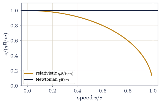
Fig. 372 The cyclotron frequency against particle speed. The Newtonian value \(qB/m\) (dark) is constant, but the relativistic frequency \(qB/(\gamma m)\) (amber) falls as \(1/\gamma\), dropping toward zero as \(v\to c\). A cyclotron driven at the fixed Newtonian frequency loses sync with the particle as it speeds up — the failure that forced the invention of the synchrocyclotron and synchrotron.#
Exercise 5 — Crossed fields and the E×B drift (worked)#
When \(\mathbf E\) and \(\mathbf B\) are perpendicular, something elegant happens: superposed on the circular gyration, the guiding center drifts sideways at a constant velocity \(\mathbf v_{\rm drift}=(\mathbf E\times\mathbf B)/B^2\) Eq. 369, of magnitude \(E/B\) and — remarkably — independent of the particle’s charge and mass. Electrons and protons drift together, which is why the \(\mathbf E\times\mathbf B\) drift is foundational in plasma physics. The trajectory is a cycloid: a fast little circle carried along by the steady drift (Fig. 373).
The fields below are \(\mathbf E=10^6\,\)V/m along \(y\) and \(\mathbf B=0.1\,\)T along \(z\), so \(E/B=10^7\,\)m/s — well below \(c\), which keeps the drift a drift rather than a runaway — and \(\mathbf E\times\mathbf B\) points along \(+x\). Averaging the velocity over whole gyro-orbits is what isolates the guiding centre: the circular part integrates to zero over a period, leaving only the steady sideways motion.
Part a) Integrate a proton starting from rest in those crossed fields over four
gyroperiods with solve_ivp (DOP853), driven by the lorentz_rhs you wrote in
Exercise 3.
Part b) Confirm its mean velocity — the drift — equals \((\mathbf E\times\mathbf B)/B^2\) in both direction and magnitude \(E/B\).
Part c) Draw the cycloid against the predicted drift displacement (Fig. 373).
E = 1e+06 V/m (y), B = 0.1 T (z),  E/B = 1.00e+07 m/s
predicted drift (E×B)/B² = [10000000.        0.        0.] m/s
measured mean velocity   = [1.00117017e+07 2.45800000e+02 0.00000000e+00] m/s
drift magnitude 1.001e+07 m/s  vs  E/B = 1.000e+07 m/s
Validation 5#
✓ the measured drift equals (E×B)/B² in direction and magnitude E/B [max|Δ| = 11701.7 (rtol=0.01, atol=100000)]
True
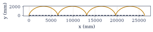
Fig. 373 A proton in crossed \(\mathbf E\) (along \(y\)) and \(\mathbf B\) (along \(z\)) fields, starting from rest. The path is a cycloid: the magnetic field curls the motion into successive arches, while the combination drives a steady drift at \(\mathbf v=(\mathbf E\times\mathbf B)/B^2\) (here along \(+x\), dashed), of magnitude \(E/B=10^7\,\)m/s. The drift is independent of the charge and mass, so every species drifts together — a cornerstone of plasma physics.#
Exercise 6 — A relativistic charge accelerated by E (student)#
A constant electric field exerts a constant force, and in Newtonian mechanics that means a constant acceleration and a speed growing without bound. Relativity forbids the latter: the force still adds momentum at a constant rate, so \(p=qEt\) grows linearly forever, but the speed recovered from that momentum saturates at \(c\) and never reaches it (Fig. 374). This is the dynamical speed limit of §4.5 seen as a trajectory — the energy cost of the last increment of speed diverges, even though nothing stops us pushing.
The run below uses \(\mathbf E=10^7\,\)V/m and follows the proton for thirty times the characteristic time \(mc/qE\) at which the momentum reaches \(mc\) — long enough for the Newtonian prediction \(v=qEt/m\) to have sailed far past \(c\) while the true speed is still creeping up on it.
Part a) Integrate a proton starting from rest in that field with solve_ivp (DOP853),
driven by the lorentz_rhs you wrote in Exercise 3.
Part b) Confirm the integrated momentum matches the exact constant-force law \(p=qEt\) at every step.
Part c) Confirm with a numpy comparison that the final speed is very close to but
below \(c\), while the momentum has grown far beyond \(mc\) and is still climbing linearly.
final speed v = 0.99944 c  (below c)
final momentum p = 30.0 mc  (and still growing linearly)
speed asymptotes to c while momentum grows without bound: True
Validation 6#
✓  a constant force adds momentum at a constant rate — the integrated p equals qEt exactly   [max|Δ| = 6.16298e-33 (rtol=1e-08, atol=1e-09)]
✓  a constant force accelerates a charge toward c but never to it — p grows unbounded, v saturates
True
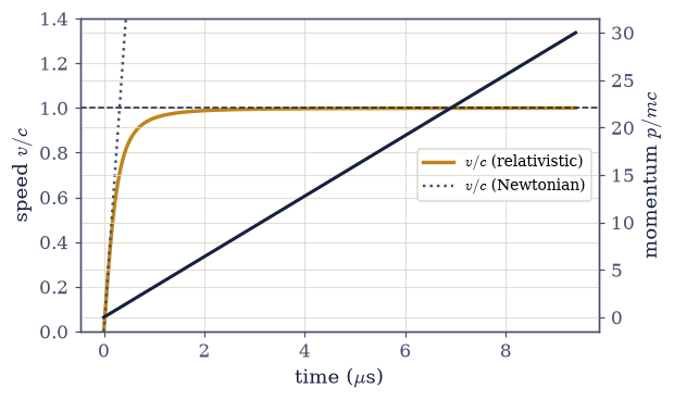
Fig. 374 A proton from rest in a uniform electric field. The momentum \(p=qEt\) (dark, right axis) grows linearly without bound, exactly as a constant force demands. But the speed \(v\) (amber, left axis) recovered from that momentum saturates at \(c\) (dashed), approaching but never reaching it, where the Newtonian prediction \(v=qEt/m\) (dotted) would sail straight past. The dynamical speed limit of §4.5, seen along a trajectory.#
Exercise 7 — Noether for the relativistic particle (student)#
Volume II’s Noether theorem (§2.2) ties each continuous symmetry of the action to a conserved quantity, and the relativistic free particle is no exception. Its Lagrangian \(L=-mc^2\sqrt{1 -v^2/c^2}\) has no explicit dependence on time or position, so time-translation symmetry conserves the energy \(\gamma mc^2\) and space-translation symmetry conserves the momentum \(\gamma m\mathbf v\) Eq. 365 — together, the conservation of four-momentum that §4.5 asserted. We confirm it directly along an integrated free trajectory.
The trajectory is a free proton at \(\mathbf v=(0.5,0.3,0)c\), followed for \(10^{-7}\,\)s with both fields set to zero. The integrator tolerances are one notch tighter than the working defaults, because the conservation is graded at \(10^{-8}\) and the only possible source of drift here is the integrator, not the physics.
Part a) Integrate that free proton with solve_ivp (DOP853), driven by the
lorentz_rhs you wrote in Exercise 3 with both field arguments zero.
Part b) Confirm with numpy that the energy \(\gamma mc^2\), recovered along the
worldline from \(E=\sqrt{(pc)^2+(mc^2)^2}\), stays constant — time-translation symmetry.
Part c) Confirm that the momentum \(\gamma m\mathbf v\) stays constant too — Noether’s theorem made numerical.
free proton at v = (0.5, 0.3, 0)c
energy: spread 1.40e-16 (relative)  → conserved
momentum p_x: spread 1.56e-16 (relative)  → conserved
Validation 7#
✓  Noether: time-translation symmetry conserves the energy γmc²   [max|Δ| = 0 (rtol=1e-08, atol=1e-09)]
✓  Noether: space-translation symmetry conserves the momentum γmv   [max|Δ| = 0 (rtol=1e-08, atol=1e-09)]
True
Exercise 8 — One mechanics, one electrodynamics, made relativistic#
Look at what has converged in this notebook. Volume II’s variational mechanics found its relativistic form in an action that is nothing but the proper time, handing back the four-momentum of §4.5 and, through Noether, its conservation. Volume III’s electrodynamics found its dynamical form in the covariant Lorentz force \(dp^\mu/d\tau=qF^{\mu\nu}u_\nu\), the field tensor of §3.12 now setting a charge in motion. The four-vectors of §4.3, the four-momentum of §4.5, the field tensor of §3.12, and the Noether theorem of §2.2 are not separate results but one structure seen from different sides. And the central idea — that a free particle extremizes its proper time — is the seed of the capstone: in curved spacetime, extremizing proper time becomes motion along geodesics, which is gravity itself.
The closing check is the unifying one, and it is stronger than any single case: the three configurations below — pure \(\mathbf E\), pure \(\mathbf B\), and crossed fields — exercise every slot of the tensor packing in turn, so a sign misplaced anywhere in it would show up in at least one of them. The test velocity is \(\mathbf v=(0.3,0.2,0.1)c\), generic enough that no component of \(\mathbf v\times\mathbf B\) vanishes by accident.
Part a) For each configuration, contract \(qF^{\mu\nu}u_\nu\) from the Setup’s
field_tensor and confirm with np.allclose that it reproduces the elementary
\(q(\mathbf E+\mathbf v\times\mathbf B)\) — one equation of motion underlying every case in
this notebook.
  pure E  : covariant force = elementary Lorentz force → True
  pure B  : covariant force = elementary Lorentz force → True
  crossed : covariant force = elementary Lorentz force → True

one covariant law reproduces every case: True
Validation 8#
✓ one covariant force law (from the §3.12 field tensor) underlies every field configuration
True
Notebook summary#
The free relativistic Lagrangian Eq. 364, Eq. 365: \(L=-mc^2\sqrt{1-v^2/c^2}\) is (minus) the proper time, so extremizing the action extremizes proper time (the result of §4.4 as a variational principle); \(\partial L/\partial v=\gamma mv\) (symbolic and finite-difference) and \(pv-L=\gamma mc^2\) recover the four-momentum of §4.5.
The covariant Lorentz force Eq. 367: \(dp^\mu/d\tau=qF^{\mu\nu}u_\nu\), built from the field tensor of §3.12 and contracted with
np.einsum, reproduces \(q(\mathbf E+ \mathbf v\times\mathbf B)\) in its spatial part and the power \(q\mathbf E\cdot\mathbf v\) in its time part — the Volume III \(\leftrightarrow\) IV handshake.Relativistic cyclotron Eq. 368: the orbit is circular with conserved speed, and the frequency measured from integrated orbits at \(\beta=0.1\)–\(0.9\) is \(\omega=qB/(\gamma m)\), the Newtonian \(qB/m\) divided by \(\gamma\) — the falloff that doomed the fixed-frequency cyclotron and forced the synchrotron.
Crossed fields Eq. 369: the guiding center drifts at \((\mathbf E\times\mathbf B)/ B^2\), magnitude \(E/B=10^7\,\)m/s, independent of charge and mass — the plasma-physics drift.
The dynamical speed limit and Noether: a constant \(\mathbf E\) grows \(p=qEt\) without bound while \(v\to c\) (§4.5 as a trajectory); and the free particle conserves \(\gamma mc^2\) and \(\gamma m\mathbf v\) by Noether’s theorem (§2.2).
Variational mechanics (II) and electrodynamics (III), both made relativistic, meet in one action and one covariant force.
Outlook#
The general-relativity capstone (§4.8). Extremizing proper time in curved spacetime is geodesic motion — gravity as geometry. The free-particle action here is the flat-spacetime seed of it.
Particle accelerators. The synchrotron that the cyclotron’s \(1/\gamma\) falloff demanded, and synchrotron radiation (a callback to §3.10).
Plasma physics. Guiding-center drifts and magnetic mirrors, built on the \(\mathbf E \times\mathbf B\) drift (a pointer).
Classical field theory. The field Lagrangian and the action for the electromagnetic field itself (Landau & Lifshitz) — a pointer beyond the course.
Cross-reference §2.1/§2.2 (Lagrangian mechanics and Noether), §3.12 (the field tensor), and §4.5 (four-momentum).