


5.14 Heat Engines and Thermodynamic Cycles#
Notebook overview#
Thermodynamics did not begin with entropy; it began with an engineering question. Sadi Carnot asked in 1824 [Car24] how much work a steam engine could possibly extract from a given flow of heat, and his answer — a bound that depends only on two temperatures, not on the working substance, the pressure, or the cleverness of the design — is among the most consequential single results in physics. This volume has so far run the logic the modern way, from microstates to entropy to free energies (§5.4, §5.7); this notebook closes the loop and spends that machinery on the subject it was invented for.
The plan is to build the cycles, leg by quadrature-checked leg, on the ideal gas whose every property §5.6 certified. Carnot’s cycle delivers its bound exactly; the Otto cycle prices the engine in every car; the same arithmetic run backwards explains why a heat pump beats a resistance heater several times over. And because the course prizes honesty about idealization, the finale is the endoreversible engine of Curzon and Ahlborn [CA75]: let the heat flow through finite conductances — as it must in any machine that runs at nonzero power — and the efficiency at maximum power drops from Carnot’s \(1 - T_c/T_h\) to the startling \(1 - \sqrt{T_c/T_h}\), a formula with no adjustable constants that lands within a few points of real coal, nuclear, and geothermal plants. The volume’s standing reference remains [Nol18].
A note on reading the checks in this notebook: a validation compares a result to an expected physical fact. A ✗ does not by itself mean the answer is wrong; it means the output did not match what the check expected, which may be a genuine error, a different-but-valid convention, or too tight a tolerance. Treat a ✗ as a prompt to locate the discrepancy. Passing is strong evidence, not proof.
Theory in brief#
The working substance. Throughout, the working gas is the monatomic ideal gas of §5.6 in units \(Nk_B = 1\): equation of state \(pV = T\), internal energy \(U = \tfrac32 T\), adiabatic index \(\gamma = 5/3\), and entropy (up to a constant) \(S = \tfrac32\ln T + \ln V\). Quasi-static work is \(W = \int p\,dV\), and the first law \(\Delta U = Q - W\) prices every leg of every cycle. Two leg types recur: the isotherm, along which \(\Delta U = 0\) so \(Q = W = T\ln(V_f/V_i)\), and the adiabat, along which \(Q = 0\), \(TV^{\gamma-1}\) is constant, and \(W = -\Delta U = \tfrac32(T_i - T_f)\).
The Carnot cycle and the bound. Two isotherms at \(T_h\) and \(T_c\) joined by two adiabats. Because heat enters only at \(T_h\) and leaves only at \(T_c\), the entropy bookkeeping is a rectangle in the \(T\)–\(S\) plane, and the efficiency \(\eta = W_{\rm net}/Q_h\) is
independent of everything but the two reservoir temperatures. The second law forbids any engine between the same reservoirs from doing better; the \(T\)–\(S\) rectangle makes the geometry of the claim visible (net work = enclosed area, in either the \(p\)–\(V\) or the \(T\)–\(S\) plane).
The Otto cycle. Two adiabats joined by two isochores (constant volume) — the idealization of the spark-ignition engine, where the compression ratio \(r = V_{\max}/V_{\min}\) is the design parameter. Working the four legs gives
with \(\gamma \approx 1.4\) for the air the real engine breathes.
Refrigerators and heat pumps. Run any engine backwards and work pumps heat uphill. The figure of merit is the coefficient of performance: for a refrigerator \({\rm COP}_{\rm fr} = Q_c/W\), for a heat pump \({\rm COP}_{\rm hp} = Q_h/W\), with the reversible (Carnot) limits
the last identity being the first law wearing a party hat: every joule of work ends up as delivered heat too.
Endoreversibility: the Curzon–Ahlborn square root. Carnot’s engine attains its bound only reversibly — infinitely slowly, at zero power. A real plant must push heat through finite thermal conductances, so the working fluid runs hotter than the cold reservoir and colder than the hot one (\(T_c < T_{cw} < T_{hw} < T_h\)), reversible inside, irreversible at the contacts. Maximizing the power rather than the efficiency over the intermediate temperatures gives, remarkably independently of the conductances,
Curzon and Ahlborn’s result [CA75] (anticipated by Novikov and by Chambadal in the 1950s). It is the rare formula that improves on an exact bound as a description of reality: real plants are built to maximize power per dollar, not efficiency, and their observed efficiencies track Eq. 459 far better than Eq. 456.
Setup#
Data only: the working substance, and nothing that assembles it into a cycle. The gas is the monatomic ideal gas of §5.6 in \(Nk_B = 1\) units, with \(\gamma = 5/3\) except where the Otto cycle breathes diatomic air (\(\gamma = 1.4\)), stated where used. The three functions below are the equations of state the theory above already displays, typed out one line each: the isotherm \(p = T/V\), the adiabat with \(pV^\gamma\) constant, and the entropy \(S = \tfrac32\ln T + \ln V\). They are the substance the problem hands us, not machinery anyone builds. Every cycle in this notebook is assembled from them inside its own exercise, and the assemblies that deserve a name are written there: the Otto leg march in Exercise 2, the endoreversible model in Exercise 4, the Stirling path in Exercise 5. Nothing in this notebook is stochastic.
The Setup below holds this notebook’s data and instruments — nothing you are asked to build. It is collapsed so the building stays yours; expand it whenever you want the details.
Exercise 1 — The Carnot cycle, leg by leg#
The bound Eq. 456 deserves to be earned, not quoted, and quadrature can do the accounting one leg at a time. Take \(T_h = 500\), \(T_c = 300\), and the hot isotherm running from \(V_1 = 1\) to \(V_2 = 2\); the two adiabats then fix \(V_3 = V_2 (T_h/T_c)^{3/2}\) and \(V_4 = V_1 (T_h/T_c)^{3/2}\) (from \(TV^{\gamma-1}\) constant with \(\gamma = 5/3\)). The closed forms each leg is cast against are the ones named in the theory above: \(T\ln(V_f/V_i)\) for an isotherm, and \(W = \tfrac32(T_i - T_f)\) for an adiabat, which is the first law with \(\Delta U = \tfrac32 \Delta T\) and \(Q = 0\). Only heat taken in counts in the denominator of \(\eta = W_{\rm net}/Q_h\), and on an isotherm \(Q = W\), so \(Q_h\) is the hot leg’s work alone. Summed around the loop the net work should come to \((T_h - T_c)\ln(V_2/V_1) = 138.629\), which is also the area \((T_h - T_c)\,\Delta S\) of the \(T\)–\(S\) rectangle whose width is the hot isotherm’s entropy change \(\Delta S = \ln(V_2/V_1)\).
Part a) Compute the work of each leg and their sum: the two
isothermal legs by scipy.integrate.quad of \(p(V) = T/V\), the two
adiabatic legs from the first law.
Part b) Verify the leg accounting: each isothermal quadrature
against its closed form (rtol=1e-10), the two adiabatic works
cancelling exactly, and the net work equal to \(138.629\).
Part c) Verify that the bound is attained and that the geometry
says the same thing: \(\eta = W_{\rm net}/Q_h\) equals \(1 - T_c/T_h = 0.4\)
(rtol=1e-12), the \(T\)–\(S\) rectangle’s area (built from entropy_ideal)
reproduces the net work (rtol=1e-12), and entropy returns exactly to
its starting value around the loop (atol=1e-14): the state function
came home.
Part d) Draw the cycle in both planes: the \(p\)–\(V\) loop (isotherms and adiabats as curves, the enclosed area shaded) beside the \(T\)–\(S\) rectangle. One irregular loop and one rectangle, the same area: the \(T\)–\(S\) plane is where Carnot’s argument lives.
legs: W_hot 346.5736, W_ad 300.0/-300.0, W_cold -207.9442
W_net = 138.629436 T–S area = 138.629436
eta = 0.400000000000 (1 - Tc/Th = 0.400000000000)
entropy around the loop: 0.00e+00
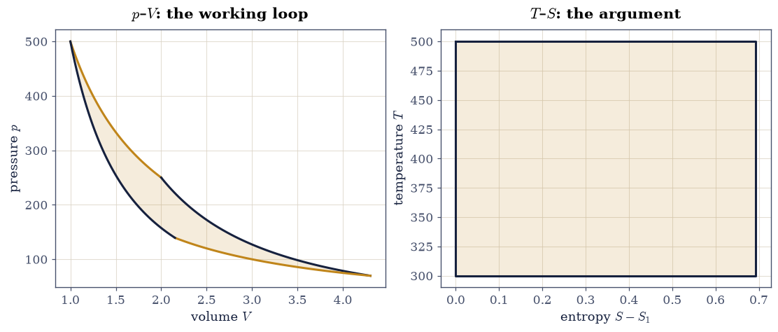
Fig. 478 The Carnot cycle for the monatomic ideal gas (\(T_h=500\), \(T_c=300\), \(V_1=1\), \(V_2=2\), units \(Nk_B=1\)) drawn in the \(p\)–\(V\) plane (left: isotherms in amber, adiabats in ink, enclosed area shaded) and in the \(T\)–\(S\) plane (right: a rectangle of height \(T_h-T_c\) and width \(\Delta S=\ln 2\)). The two shaded areas are equal — both are the net work \(138.63\) — but only the rectangle makes the efficiency bound legible at a glance.#
✓ quadrature of p = T/V reproduces the closed-form isothermal work T ln(V2/V1) [got 346.574 vs expected 346.574 (rtol=1e-10, atol=1e-09)]
✓ the two adiabatic works cancel exactly: what the expansion gives, the compression takes back [sum = 0.0e+00]
✓ the constructed cycle attains Carnot's bound 1 - Tc/Th = 0.4 exactly [got 0.4 vs expected 0.4 (rtol=1e-12, atol=1e-09)]
✓ and the T–S rectangle's area IS the net work: the geometric form of the argument [got 138.629 vs expected 138.629 (rtol=1e-12, atol=1e-09)]
✓ entropy returns exactly around the loop: a state function came home [loop sum 0.0e+00]
True
Exercise 2 — The Otto cycle: the engine in the driveway#
Eq. 457 prices every spark-ignition engine. The idealized cycle: adiabatic compression from \(V_{\max}\) to \(V_{\min}\) (the piston rising), isochoric heat injection at \(V_{\min}\) (the spark), adiabatic expansion back to \(V_{\max}\) (the power stroke), isochoric heat rejection (the exhaust). Take compression ratio \(r = 10\), air (\(\gamma = 1.4\)), intake at \(T_1 = 300\), and a spark that heats the compressed gas by \(\Delta T = 1500\) (with \(c_V = 1/(\gamma - 1) = 2.5\) in these units). Both isochoric legs exchange heat at constant volume, so each costs \(c_V\) times its temperature change, and the adiabatic strokes carry no heat at all; the corners therefore follow from \(T V^{\gamma-1}\) constant alone. The compression ratio turns out to be the whole game — which is why diesels, running higher \(r\), are more efficient. Real engines, though, deliver roughly \(0.25\)–\(0.35\) rather than the ideal \(0.60\): friction, finite-time combustion, heat loss through cylinder walls, and the impossibility of truly adiabatic strokes all take their cut. Idealized cycles are bounds and design compasses, not predictions, and the endoreversible engine of Exercise 4 begins to close that gap.
Part a) Write otto_efficiency(dT_spark): march through the four
corners with the adiabatic relation \(T V^{\gamma-1}\) constant, form
\(Q_{\rm in} = c_V\,\Delta T\) and \(Q_{\rm out} = c_V (T_4 - T_1)\), and
return \(1 - Q_{\rm out}/Q_{\rm in}\). Write this one yourself — the
implementation is the lesson.
Part b) Verify that this leg-by-leg efficiency equals the closed
form \(1 - r^{1-\gamma} = 0.6019\) to rtol=1e-12, and that it does not
depend on \(\Delta T\): the same efficiency (to rtol=1e-12) comes back
at \(\Delta T = 800\).
Part c) Verify that the idealization gap is large: the ideal \(0.6019\) exceeds a representative real value \(0.30\) by more than \(80\%\) of the latter.
eta (ΔT=1500): 0.601893
eta (ΔT=800) : 0.601893
closed form : 0.601893
real engines : ~0.3
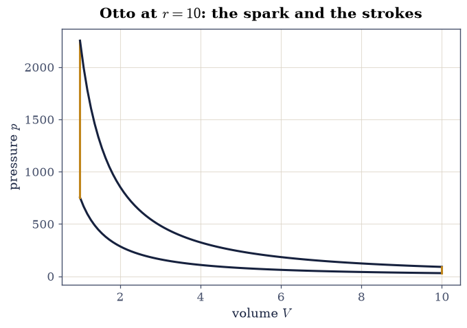
Fig. 479 The idealized Otto cycle in the \(p\)–\(V\) plane for compression ratio \(r=10\) and air (\(\gamma=1.4\)): adiabatic compression (ink, 1→2), isochoric spark (amber, 2→3), adiabatic power stroke (ink, 3→4), isochoric exhaust (amber, 4→1), with intake at \(T_1=300\) and a \(\Delta T=1500\) spark. The efficiency \(1-r^{1-\gamma}=0.602\) depends only on the compression ratio — not on how hard the spark heats — which is the design logic of every engine in every driveway.#
✓ the four legs assemble to the closed form 1 - r^(1-γ) = 0.602 [got 0.601893 vs expected 0.601893 (rtol=1e-12, atol=1e-09)]
✓ and the spark strength drops out entirely: the compression ratio is the whole game [got 0.601893 vs expected 0.601893 (rtol=1e-12, atol=1e-09)]
✓ the idealization gap is large: real engines deliver about half the ideal figure — bounds are not predictions [0.602 vs ~0.3]
True
Exercise 3 — Backwards: refrigerators and the heat-pump bargain#
Reverse the cycle and work pumps heat from cold to hot; Eq. 458 prices it. A kitchen refrigerator holds its interior at \(T_c = 275\ \mathrm K\) against a room at \(T_h = 295\ \mathrm K\); a heat pump warms the same room against the same \(20\ \mathrm K\) gap. A heat pump delivering \(Q_h\) uses \(Q_h/{\rm COP}\) of work while a resistance heater uses \(Q_h\) outright, so the COP is exactly the factor by which the pump beats the resistor. Real machines run a seasonal COP near \(3.5\) against that reversible \(14.75\) — the usual factor-of-four honesty gap — and cold climates make it worse, because the denominator of Eq. 458 is the temperature gap itself.
Part a) Compute the reversible \({\rm COP}_{\rm fr}\) and \({\rm COP}_{\rm hp}\) for the \(20\ \mathrm K\) gap, and the reversible \({\rm COP}_{\rm hp}\) once more at an outdoor temperature of \(255\ \mathrm K\) (\(-18\ \mathrm{^\circ C}\)).
Part b) Verify the reversible figures: \({\rm COP}_{\rm fr} =
275/20 = 13.75\) and \({\rm COP}_{\rm hp} = 295/20 = 14.75\)
(rtol=1e-12 each), and the first-law identity \({\rm COP}_{\rm hp} -
{\rm COP}_{\rm fr} = 1\) exactly (atol=1e-12): the work you pay
arrives in the room as heat, every joule of it.
Part c) Verify the bargain and its honest size: the real \(3.5\)
still heats the room with \(3.5\times\) less electricity than the
resistor while sitting a factor \(\sim 4\) below its own reversible
bound, and the winter figure is \(7.375\) — exactly half of \(14.75\)
(rtol=1e-12), because the gap doubled. Pumping uphill costs in
proportion to the hill.
COP fridge (reversible) : 13.7500
COP heat pump (reversible): 14.7500
identity COP_hp - COP_fr : 1.000000000000
winter (255 K outdoors) : 7.3750
real seasonal COP ~ 3.5: heat for 0.29 of the resistor's electricity
✓ the reversible coefficients: 13.75 to keep the milk cold, 14.75 to warm the room [max|Δ| = 0 (rtol=1e-12, atol=1e-09)]
✓ COP_hp - COP_fr = 1 exactly: the paid work arrives as heat too [difference 1.000000000000]
✓ even a real heat pump beats resistance heating 3.5-fold, while sitting a factor ~4 below its reversible bound [real 3.5 vs reversible 14.75]
✓ and doubling the temperature gap exactly halves the reversible COP: pumping uphill costs in proportion to the hill [got 2 vs expected 2 (rtol=1e-12, atol=1e-09)]
True
Exercise 4 — The Curzon–Ahlborn engine: power against perfection#
Now the finale’s physics, modelled the way Curzon and Ahlborn modelled it [CA75]: a Carnot engine runs reversibly between internal temperatures \(T_{hw}\) and \(T_{cw}\), while the heat it uses must leak in and out through finite conductances from the true reservoirs at \(T_h\) and \(T_c\). In the steady state the reversible core forces the entropy balance \(Q_h/T_{hw} = Q_c/T_{cw}\), and with Newton’s-law heat flow (\(Q \propto\) temperature drop) the power \(P = Q_h - Q_c\) becomes a function of a single free internal temperature. Take the two conductances equal and absorb them into the units, so that \(Q_h = T_h - T_{hw}\) and \(Q_c = T_{cw} - T_c\); the entropy balance then reads \(T_c = T_{cw}(1 - Q_h/T_{hw})\), which is what fixes \(T_{cw}\) from a trial \(T_{hw}\). Trial temperatures that break the ordering \(T_c < T_{cw} < T_{hw} < T_h\) describe no engine at all, and are best reported as zero power so the maximizer simply avoids them. The internally reversible core runs at \(\eta = 1 - T_{cw}/T_{hw}\), between the internal temperatures rather than the reservoir ones.
Part a) Write ca_power_and_eta(T_hw, T_h, T_c), returning the
power and the efficiency of the endoreversible engine at internal
temperature \(T_{hw}\). Write this one yourself — the implementation
is the lesson.
Part b) Maximize the power over \(T_{hw} \in (T_c, T_h)\) with
scipy.optimize.minimize_scalar (bounded) at \(T_h = 500\), \(T_c = 300\),
and verify the efficiency at maximum power equals the closed form
\(1 - \sqrt{T_c/T_h} = 0.22540\) to rtol=1e-5 — the square root
emerging from an optimization that never mentions it — and that it sits
well below Carnot’s \(0.4\): the price of running at nonzero power.
Part c) The confrontation with reality, using Curzon and Ahlborn’s own comparison set: the West Thurrock coal station (\(T_h = 838\), \(T_c = 298\ \mathrm K\), observed \(\eta = 0.36\)), the CANDU nuclear reactor (\(573\), \(298\), observed \(0.30\)), and the Larderello geothermal field (\(523\), \(353\), observed \(0.16\)). Verify that for all three, \(|\eta_{\rm CA} - \eta_{\rm obs}| < 0.05\) while Carnot overshoots by more than \(0.15\) for the two steam plants: a zero-parameter formula out-predicting an exact bound, because it asks the question the engineers asked.
West Thurrock (coal) Carnot 0.644 CA 0.404 observed 0.36
CANDU (nuclear) Carnot 0.480 CA 0.279 observed 0.30
Larderello (geothermal) Carnot 0.325 CA 0.178 observed 0.16
eta at max power (numeric): 0.225403 (1 - √(Tc/Th) = 0.225403)
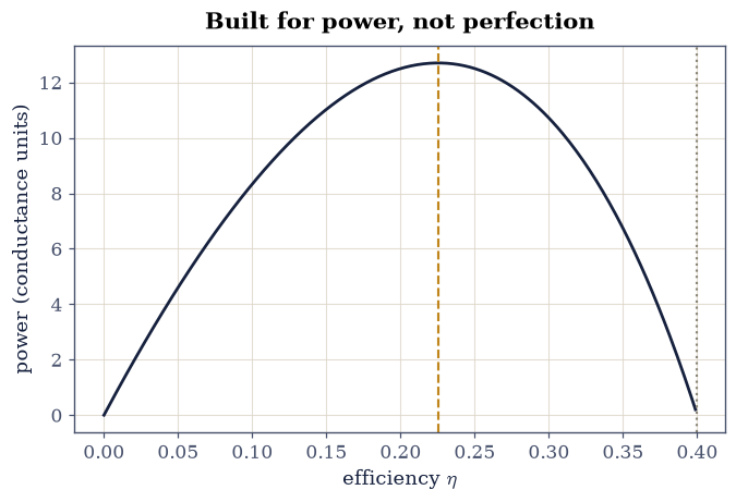
Fig. 480 Power against perfection: the endoreversible engine’s output power (in conductance units) against its efficiency, traced by sweeping the internal hot-side temperature between the reservoirs at \(T_h=500\) and \(T_c=300\). Power vanishes at both ends — at \(\eta=0\) (all drop wasted across the contacts) and at Carnot’s \(\eta=0.4\) (reversible, hence infinitely slow) — and peaks at exactly \(\eta_{\rm CA}=1-\sqrt{T_c/T_h}=0.225\) (dashed): the efficiency real machines are built near, because they are built for power.#
✓ maximizing POWER over the internal temperatures lands on 1 - √(Tc/Th): the square root emerges from an optimization that never mentions it [got 0.225403 vs expected 0.225403 (rtol=1e-05, atol=1e-09)]
✓ and it sits far below Carnot: the price of running at nonzero power [0.225 vs Carnot 0.400]
✓ Curzon–Ahlborn lands within 0.05 of all three real plants — coal, nuclear, geothermal — with zero adjustable parameters [deviations [np.float64(0.044), np.float64(0.021), np.float64(0.018)]]
✓ while Carnot overshoots the two steam plants by more than 15 points: the exact bound answers a question nobody built for [Carnot excesses [0.284, 0.18, 0.165]]
True
Exercise 5 — The Stirling cycle and the regenerator’s trick#
One more cycle earns its place, both for its geometry and for its moral. The Stirling cycle joins two isotherms by two isochores: heat the gas at constant \(V_1\), expand isothermally at \(T_h\), cool at constant \(V_2\), compress isothermally at \(T_c\). Run naively, the isochoric legs draw heat at temperatures below \(T_h\), so the efficiency falls short of Carnot. The regenerator — Robert Stirling’s 1816 trick, decades before thermodynamics existed — stores the isochoric-cooling heat in a thermal labyrinth and returns exactly the same amount during isochoric heating (the two legs span the same temperature interval, so the exchange balances identically). With the isochoric heats internalized, only the isotherms touch the reservoirs, and Carnot efficiency returns.
The working numbers are \(T_h = 500\), \(T_c = 300\), \(V_1 = 1\), \(V_2 = 2\) and a monatomic gas (\(c_V = 3/2\)), the same reservoirs and the same \(\Delta S\) as the Carnot cycle of Exercise 1, so its net work \((T_h - T_c)\ln 2 = 138.63\) should reappear here unchanged. Each isotherm exchanges \(T\ln(V_2/V_1)\) and each isochore \(\tfrac32(T_h-T_c)\), with signs set by direction. Bought naively, the denominator of the efficiency is everything the cycle draws in, isochoric heating included; with the regenerator, it is the hot isotherm alone.
Part a) Price the four legs and form both efficiencies, the naive \(W/(Q_{\rm isotherm} + Q_{\rm isochore})\) and the regenerated \(W/Q_{\rm isotherm}\).
Part b) Verify the net work is \(138.63\), identical to Exercise 1’s
(rtol=1e-12), and that the naive efficiency is \(0.2144\) (rtol=1e-4),
well below Carnot’s \(0.4\).
Part c) Verify the regenerator’s exchange balances exactly — the
isochoric heats are equal and opposite (atol=1e-12) — and that with
them internalized the efficiency is exactly Carnot’s \(1 - T_c/T_h\)
(rtol=1e-12). A cycle whose legs are humbler than Carnot’s reaches
the same bound by clever bookkeeping: the second law cares only about
where entropy crosses the boundary.
Part d) Draw the cycle in the \(p\)–\(V\) plane: two isotherms joined by two vertical isochores, a loop with corners where Carnot’s has none.
Part e) Animate the working loop: assemble the four legs into one closed \((V, p)\) path and send a state point around it while a bar gauge tracks the running net work \(\oint p\,dV\) by trapezoid quadrature, resetting each cycle. The animation’s physics is certified by Part a)’s leg accounting, computed from the same path the point traces.
W_net = 138.6294 (Carnot cycle's: 138.6294)
eta naive : 0.2144
eta regen : 0.4000 (Carnot 0.4000)
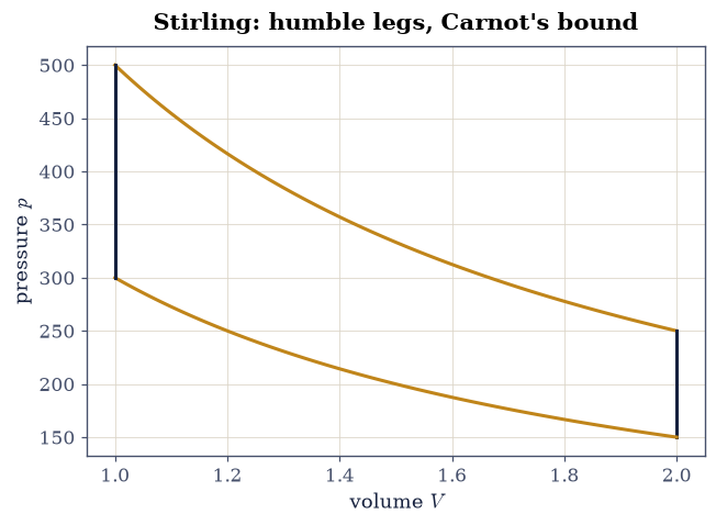
Fig. 481 The Stirling cycle (\(T_h=500\), \(T_c=300\), \(V_1=1\), \(V_2=2\), monatomic gas): two isotherms (amber) joined by two isochores (ink) in the \(p\)–\(V\) plane. Its net work equals the Carnot cycle’s between the same reservoirs, but bought naively its isochoric heating drags the efficiency to \(0.214\); with Stirling’s regenerator internalizing the exactly-balanced isochoric heats, the cycle recovers Carnot’s \(0.4\).#
✓ same reservoirs, same ΔS, same net work as the Carnot cycle of Exercise 1 [got 138.629 vs expected 138.629 (rtol=1e-12, atol=1e-09)]
✓ bought naively, the isochoric heat drags the efficiency to 0.214 [got 0.214406 vs expected 0.2144 (rtol=0.0001, atol=1e-09)]
✓ but the two isochoric heats balance exactly: the regenerator's exchange is an identity, not an approximation [sum 0.0e+00]
✓ and with them internalized the Stirling cycle attains Carnot exactly: the second law only counts entropy crossing the boundary [got 0.4 vs expected 0.4 (rtol=1e-12, atol=1e-09)]
True