2.1 Lagrangian Mechanics with SymPy

Elementary Computational Physics

Volume II — Analytical Mechanics Notebook 2.1

From a single scalar — the Lagrangian — to the equations of motion of any system, derived symbolically and integrated numerically. The workhorse tool for the rest of the series.

Level · intermediate   •   Est. · 75–100 min

Raymond Amador v1.4.0  ·  2026-07-31  ·  CC BY 4.0 (text) / MIT (code)

Notebook overview

Volume I derived equations of motion by hand and from Newton’s laws. That works for a projectile or a single pendulum, but the algebra grows vicious fast: the double pendulum of §1.3 took a page of trigonometry, and we only trusted the result because we cross-checked it against SymPy. Analytical mechanics turns that relationship around. Instead of summing forces and constraint tensions vector by vector, we write down one scalar (the Lagrangian \(\mathcal L = T - V\)) and a single mechanical recipe, the Euler–Lagrange equations, produces the equations of motion for every coordinate at once.

The recipe is pure calculus on a scalar, which means a computer algebra system can carry it out mechanically and without error. This notebook builds that tool — you write the small euler_lagrange engine in Exercise 1 and the to_numeric bridge to solve_ivp in Exercise 2 — and then puts it to work on a sequence of systems: the harmonic oscillator and the pendulum (to trust the engine against answers we know), the Atwood machine (to see a constraint vanish), the double pendulum (where the symbolic derivation becomes the primary method, with the hand algebra of §1.3 now the thing being checked), a cart-pole (painful by hand, lovely in motion), and a central-force orbit (where a cyclic coordinate hands us a conservation law for free). This engine is the workhorse we will reuse throughout Volume II and beyond.

How to read the checks. Each exercise ends with a validation that compares our result to an expected physical fact. A ✗ does not by itself mean the answer is wrong: it means the output didn’t match what the check expected, which may be a real error, a different-but-valid convention (a sign, a unit, an array order), or simply too tight a tolerance. Treat a ✗ as a prompt to locate the discrepancy; passing is strong evidence of correctness, not proof.

Scope. This is a working review, not a textbook chapter. The variational foundations are not skipped, only postponed: §2.8 opens with a calculus-of-variations primer, derives the Euler–Lagrange equation for a general functional, and identifies that equation with the one used here. For the fuller treatment (Hamilton’s principle in its own right, the boundary terms, the constrained cases), see Nolting, Theoretical Physics 2 [Nol16], and Goldstein, Poole & Safko, Classical Mechanics [GPS02].

Theory in brief

The action and Hamilton’s principle

A mechanical system described by generalised coordinates \(q_i(t)\) has a Lagrangian \(\mathcal L(q_i, \dot q_i, t)\), and the action is its time integral along a path,

(135)\[S[q] = \int_{t_1}^{t_2} \mathcal L\bigl(q_i, \dot q_i, t\bigr)\, \mathrm dt .\]

Hamilton’s principle states that the path actually taken between two fixed endpoints is a stationary point of the action: \(\delta S = 0\). This is a remarkable repackaging of mechanics: the whole of the dynamics is encoded in a single number \(S\) being extremal, with no mention of forces. The variational derivation turns \(\delta S = 0\) into a differential equation for each coordinate; §2.8 carries that derivation out for a general functional, and [GPS02, Nol16] give the textbook version.

The Euler–Lagrange equations

Requiring \(\delta S = 0\) for arbitrary variations vanishing at the endpoints yields, for each generalised coordinate \(q_i\), the Euler–Lagrange equation

(136)\[\frac{\mathrm d}{\mathrm dt}\!\left(\frac{\partial \mathcal L}{\partial \dot q_i}\right) - \frac{\partial \mathcal L}{\partial q_i} = 0 .\]

There is one such equation per coordinate, and together they are equivalent to Newton’s laws, but expressed entirely in terms of derivatives of the scalar \(\mathcal L\). No free-body diagrams, no constraint forces to resolve.

Generalised coordinates and \(\mathcal L = T - V\)

For a system with kinetic energy \(T\) and potential energy \(V\), the Lagrangian is simply their difference,

(137)\[\mathcal L = T - V ,\]

written in whatever generalised coordinates best describe the system. This freedom is the practical heart of the method. A pendulum bob is constrained to a circle; in Cartesian \((x,y)\) that constraint needs an unknown tension force, but in the single angle \(\theta\) the constraint is built into the coordinate and the tension never appears. Choosing coordinates that automatically satisfy the constraints removes the constraint forces from the problem entirely.

Conjugate momenta and cyclic coordinates

The quantity multiplying \(\dot q_i\) in the dynamics is the conjugate (or generalised) momentum

(138)\[p_i = \frac{\partial \mathcal L}{\partial \dot q_i} .\]

If \(\mathcal L\) does not depend on a coordinate \(q_i\) explicitly (such a \(q_i\) is called cyclic, or ignorable) then Eq. 136 collapses to \(\mathrm dp_i/\mathrm dt = 0\): the conjugate momentum is conserved. This is the seed of the deep link between symmetry and conservation (Noether’s theorem, §2.2): a coordinate the Lagrangian ignores corresponds to a quantity nature conserves. Translational invariance gives momentum conservation; rotational invariance (a cyclic angle) gives angular-momentum conservation.

The computational idea

Equation Eq. 136 is nothing but differentiation of a scalar followed by solving for the highest derivatives. A computer algebra system performs exactly those operations exactly: no transcription slips, no dropped terms. So the plan is: write \(\mathcal L\), let SymPy form and solve Eq. 136 for the accelerations \(\ddot q_i\), then lambdify those symbolic accelerations into a numerical right-hand side and integrate with solve_ivp. We met this idea in §1.3 as a check on a hand derivation; here it becomes the primary method.

---

Setup

Setup holds only the toolchain — SymPy for the symbolic derivation, NumPy and SciPy for the numerics, the ecp validation and animation helpers — and the one symbol every dynamical coordinate in the notebook is a function of, the time \(t\). This notebook’s own machinery is not here: you write the euler_lagrange engine in Exercise 1 and the to_numeric bridge to scipy.integrate.solve_ivp in Exercise 2, and every later exercise runs on the two of them.

The Setup below holds this notebook’s data and instruments — nothing you are asked to build. It is collapsed so the building stays yours; expand it whenever you want the details.

Show code cell source

Hide code cell source

import numpy as np
import sympy as sp
from scipy.integrate import solve_ivp
import matplotlib.pyplot as plt
from matplotlib.animation import FuncAnimation

from ecp import validate
from ecp.animate import show

# data: the time variable shared by all dynamical coordinates
t = sp.symbols("t")

Exercise 1 — Build the Euler–Lagrange engine

The whole notebook rests on one function. The Euler–Lagrange equation Eq. 136 is, per coordinate, \(\frac{\mathrm d}{\mathrm dt}(\partial \mathcal L/\partial \dot q) - \partial \mathcal L/\partial q = 0\); SymPy can form each piece with sp.diff and solve the resulting set for the accelerations. The right way to trust a new symbolic tool is to run it on a system whose answer we already know cold — the simple harmonic oscillator, whose Lagrangian Eq. 137 is \(\mathcal L = \tfrac12 m\dot x^2 - \tfrac12 k x^2\) and whose equation of motion is Newton’s \(\ddot x = -(k/m)\,x\).

1. Write euler_lagrange(L, coords, t): form the left-hand side of Eq. 136 for each coordinate with sympy.diff and solve the coupled set for the second derivatives, returning the dict {q_i'' : expression}. Write this one yourself — the implementation is the lesson.

2. Define the symbols \(m,k\) (sympy.symbols) and the coordinate \(x(t)\) (sympy.Function), and write \(\mathcal L\).

3. Run the engine and read off \(\ddot x\); check with sympy.simplify that it equals \(-(k/m)x\).

SHO  ẍ = -k*x(t)/m

✓  the engine recovers the SHO equation of motion ẍ = -(k/m)x   [engine returned ẍ = -k*x(t)/m]

True

Exercise 2 — The simple pendulum from its Lagrangian

Now a genuinely constrained system. A pendulum bob is stuck on a circle of radius \(\ell\); in Cartesian coordinates that demands an unknown string tension, but in the single angle \(\theta\) the constraint is automatic and the tension never enters. With \(T = \tfrac12 m\ell^2\dot\theta^2\) and \(V = -mg\ell\cos\theta\) (measuring \(\theta\) from straight down), the Lagrangian Eq. 137 is \(\mathcal L = \tfrac12 m\ell^2\dot\theta^2 + mg\ell\cos\theta\).

A symbolic acceleration is also only useful once it runs as a number, so this is where the second half of the engine gets built: the bridge that turns the Euler–Lagrange accelerations into a right-hand side scipy.integrate.solve_ivp can integrate. solve_ivp wants a first-order system, so the natural packaging is the interleaved state \(y = [q_0, \dot q_0, q_1, \dot q_1, \dots]\), whose even slots are the coordinates and whose odd slots are their velocities.

1. Write \(\mathcal L\) in \(\theta\) and run the euler_lagrange you wrote in Exercise 1; confirm via Eq. 136 that \(\ddot\theta = -(g/\ell)\sin\theta\), with no tension in sight.

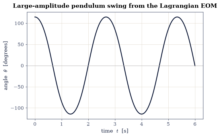
2. Write to_numeric(acc_dict, coords, t, param_values): substitute the numeric parameter values, sympy.lambdify each acceleration in acc_dict against the coordinates, their first derivatives and the parameters, and return the first-order right-hand side rhs(t, y) on the interleaved state above. Write this one yourself — the implementation is the lesson.

3. Integrate one large-amplitude swing, released from \(\theta=2.0\) rad at rest, with scipy.integrate.solve_ivp (DOP853, rtol=1e-11, atol=1e-12) over a dense t_eval; plot \(\theta(t)\).

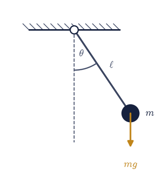
Fig. 114 The simple pendulum as a constrained system: a bob of mass \(m\) is confined to a circle of radius \(\ell\) and located by the single angle \(\theta\) from the downward vertical (dashed), under gravity \(mg\); in this generalized coordinate the constraint is automatic and the string tension never enters the Lagrangian.

pendulum  θ̈ = -g*sin(theta(t))/l

✓  pendulum EOM is θ'' = -(g/l) sinθ   [engine returned θ̈ = -g*sin(theta(t))/l]

True

Exercise 3 — A constrained system made easy: the Atwood machine

The Atwood machine (two masses \(m_1, m_2\) hanging over a frictionless pulley on an inextensible string) is the textbook case for seeing a constraint disappear. The Newtonian route introduces the string tension \(T\) as an unknown and needs two equations to eliminate it. The Lagrangian route uses one generalised coordinate \(s\), the length of string on mass \(m_1\)’s side: if \(m_1\) descends by \(s\), then \(m_2\) rises by \(s\), so the inextensible-string constraint is already encoded. The tension never appears.

Your task. With both masses moving at speed \(\dot s\), the kinetic energy is \(T = \tfrac12(m_1+m_2)\dot s^2\) and the potential is \(V = -m_1 g s + m_2 g s\) (heights \(\mp s\)). Form \(\mathcal L = T - V\), run the euler_lagrange engine you wrote in Exercise 1, and confirm the classic result \(\ddot s = (m_1 - m_2)g/(m_1+m_2)\).

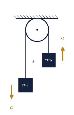
Fig. 115 The Atwood machine: masses \(m_1\) and \(m_2\) hang from an inextensible rope over an ideal pulley, sharing the single coordinate \(s\) (rope displacement) and a common acceleration magnitude \(a\); the heavier \(m_1\) descends as \(m_2\) rises, the constraint reducing two bodies to one degree of freedom.

Atwood  s̈ = g*(m1 - m2)/(m1 + m2)

✓  Atwood acceleration is (m1-m2)g/(m1+m2)   [engine returned s̈ = g*(m1 - m2)/(m1 + m2)]

True

Exercise 4 — Symbolic → numeric pipeline; energy as the correctness gate

A symbolic acceleration is only useful once it runs as a number. The to_numeric bridge you wrote in Exercise 2 lambdifies the EL accelerations into a solve_ivp right-hand side; the question is whether the resulting trajectory is correct. For an autonomous conservative system the total energy \(E = T + V\) is constant, so, exactly as in Volume I, the relative drift of \(E\) along the integrated trajectory is an independent gate on the whole pipeline (derivation, lambdify, and integration together).

Your task. Take the pendulum of Exercise 2, reconstruct its energy \(E = \tfrac12 m\ell^2\dot\theta^2 - mg\ell\cos\theta\) as an array along the trajectory you already integrated, and confirm it is conserved to tight tolerance.

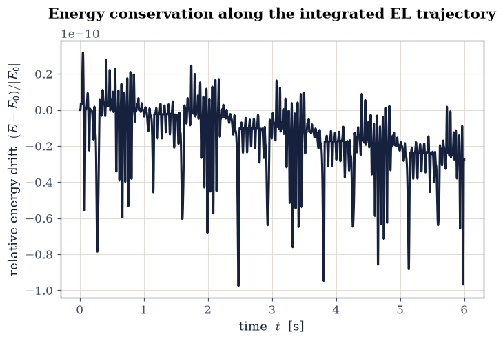
relative energy drift = 1.29e-10

✓  energy conserved along the integrated EL trajectory   [max relative drift = 9.75669e-11 (limit 1e-06)]

True

Exercise 5 — The double pendulum, derived not hand-coded (cross-check vs. 1.3)

This is the exercise that justifies the whole apparatus. In §1.3 we derived the double-pendulum equations of motion by hand: a page of trigonometry that we only trusted after checking it against SymPy. Here we invert that: the engine derives the EOM straight from the Lagrangian (the hand derivation in §1.3), and the hand-coded formula becomes the thing under test. With the bob positions \(x_1=\ell_1\sin\theta_1,\ y_1=-\ell_1\cos\theta_1\) and \(x_2=x_1+\ell_2\sin\theta_2,\ y_2=y_1-\ell_2\cos\theta_2\), the Lagrangian Eq. 137 is \(\mathcal L = T - V\) with \(T=\tfrac12 m_1(\dot x_1^2+\dot y_1^2)+\tfrac12 m_2(\dot x_2^2+\dot y_2^2)\) and \(V = m_1 g y_1 + m_2 g y_2\).

1. Build the double-pendulum Lagrangian and run the euler_lagrange you wrote in Exercise 1 to get \(\ddot\theta_1, \ddot\theta_2\) via Eq. 136.

2. Lambdify both accelerations (sympy.lambdify) and compare them to the validated hand-coded deriv from §1.3 at several random states (a seeded numpy.random.default_rng). They should agree to machine precision: the symbolic derivation reproduces the hand algebra exactly, while being immune to the slips that make hand derivations so error-prone.

max |SymPy − hand| over 8 random states = 3.55e-15

✓  SymPy double-pendulum EOM matches the validated 1.3 hand derivation   [got 3.55271e-15 vs expected 0 (rtol=1e-06, atol=1e-09)]

True

With your assistant

The symbolic boilerplate of this workflow — declaring symbols, assembling \(T\) and \(V\), wiring lambdify — is fair game to delegate: ask your assistant for the whole pipeline for a system of your choosing. The one non-negotiable step is reading the derived equation of motion line by line before you integrate it — a wrong sign in a generated Lagrangian survives every syntax check ever written and dies only under your eyes or the energy gate of Exercise 4. The check is yours.

Exercise 6 — A cart-pole, end to end (worked animation)

Now a system where the hand derivation is genuinely unpleasant but the engine shrugs: the cart-pole, a pendulum of mass \(m_p\) hanging from a cart of mass \(M\) that slides freely on a horizontal rail. The two coordinates are the cart position \(x\) and the pendulum angle \(\theta\) (from straight down); they are coupled: the swinging pole shoves the cart, the moving cart drives the pole. With the bob at \(x_p = x + \ell\sin\theta,\ y_p = -\ell\cos\theta\), the Lagrangian Eq. 137 is \(\mathcal L = \tfrac12 M\dot x^2 + \tfrac12 m_p(\dot x_p^2 + \dot y_p^2) + m_p g \ell\cos\theta\).

Note that \(x\) does not appear in \(\mathcal L\): it is cyclic Eq. 138, so the total horizontal momentum is conserved (we will return to exactly this in Exercise 7). The system is autonomous, so the total energy is conserved too, and that is what we validate. The derivation and the integration below run entirely on your Exercise 1 euler_lagrange and your Exercise 2 to_numeric — two coupled coordinates cost the engine one extra entry in coords. This is the worked animation; you build the second in Exercise 7.

The animation shows the cart sliding while the pole swings. Released nearly inverted, the pole rocks the cart back and forth.

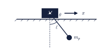
Fig. 116 The cart-pole: a cart of mass \(M\) slides without friction along a horizontal rail (its position \(x\) is the cyclic coordinate) while a pole of length \(\ell\) carrying a bob \(m_p\) swings from a hinge on the cart at angle \(\theta\) from the downward vertical (dashed), under gravity.

cart-pole energy relative drift = 1.02e-10

Once Loop Reflect

Fig. 117 Animation of the cart-pole released nearly inverted (\(\theta=2.5\) rad) with cart mass \(M=1\), pole mass \(m_p=0.3\), and length \(\ell=1\): the pole’s swings rock the freely sliding cart back and forth along the rail, the autonomous motion conserving total energy.

✓  the integrated cart-pole motion conserves total energy (autonomous system)   [max relative drift = 8.0991e-11 (limit 1e-05)]

True

Exercise 7 — Cyclic coordinate ⇒ conserved momentum (student-implemented animation)

The cart-pole hinted at it; here we make it the point. A particle of mass \(m\) moving in a central potential \(V(r)\) is best described in polar coordinates \((r,\varphi)\), with kinetic energy \(T=\tfrac12 m(\dot r^2 + r^2\dot\varphi^2)\), so the Lagrangian Eq. 137 is \(\mathcal L = \tfrac12 m(\dot r^2 + r^2\dot\varphi^2) - V(r)\). The angle \(\varphi\) does not appear (it is cyclic), so by Eq. 138 its conjugate momentum \(p_\varphi = \partial\mathcal L/\partial\dot\varphi = m r^2\dot\varphi\) is conserved. That conserved \(p_\varphi\) is the angular momentum, and its constancy is Kepler’s second law: the radius sweeps equal areas in equal times.

1. Build the central-potential Lagrangian (use \(V(r) = -k/r\)), confirm \(\partial\mathcal L/\partial\varphi = 0\) symbolically (sympy.diff), and identify \(p_\varphi = m r^2\dot\varphi\) from Eq. 138.

2. Integrate a bound orbit with your Exercise 1 euler_lagrange and your Exercise 2 to_numeric (which lambdifies the accelerations into a scipy.integrate.solve_ivp right-hand side, DOP853).

3. Build the animation of the orbiting particle with the radius vector drawn from the centre, so the equal-area sweep is visible. You have the trajectory (x, y) below; assemble a FuncAnimation showing the moving particle, its trail, and the sweeping radial line, plt.close(fig), then display with ecp.animate.show.

A ✗ on the final check is about the p_phi time series we computed from the trajectory, not the animation: any correct drawing of the same orbit is fine. If it fails, inspect \(p_\varphi(t) = m r^2\dot\varphi\) along the solution.

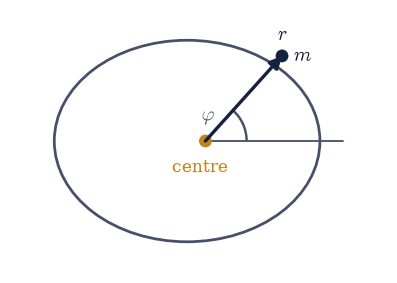
Fig. 118 Central-force geometry: a particle of mass \(m\) moves on a bound orbit about a fixed force centre (amber), located by polar coordinates \((r,\varphi)\) — radius \(r\) from the centre and azimuth \(\varphi\) from the polar axis; the angle \(\varphi\) is cyclic, so its conjugate momentum \(p_\varphi=mr^2\dot\varphi\) (the angular momentum) is conserved.

∂L/∂φ = 0   ⇒ φ is cyclic, so p_φ = m r² φ̇ is conserved
p_φ relative drift = 4.49e-11

Once Loop Reflect

Fig. 119 Animation of a bound orbit in the attractive potential \(V(r)=-k/r\) (mass \(m=1\), \(k=1\)) about the fixed force centre (grey star): the orange radius vector sweeps equal areas in equal times because the angular momentum \(p_\varphi=mr^2\dot\varphi\), conjugate to the cyclic angle \(\varphi\), is conserved (Kepler’s second law).

✓  the conjugate momentum to the cyclic coordinate φ is conserved   [max relative drift = 3.14782e-11 (limit 1e-05)]

True

Notebook summary

• A symbolic Euler–Lagrange engine built over SymPy (and packaged for the rest of the series as ecp.mechanics.euler_lagrange): the equations of motion read straight off a Lagrangian for the pendulum, the Atwood machine, the double pendulum (cross-checked against the hand-coded formula of §1.3), and a cart-pole.

• The symbolic → numeric pipeline (sympy.lambdify into scipy.integrate.solve_ivp), with energy conservation as the correctness gate, and a cyclic coordinate yielding a conserved momentum.

Outlook

• Velocity-dependent potentials. A charged particle in a magnetic field has a Lagrangian with a \(\dot{\mathbf q}\cdot\mathbf A\) term; the same engine handles it and yields the Lorentz force: a forward link to Volume III.

• When the constraint force itself is wanted. Lagrange multipliers reintroduce the constraint (and its force) explicitly: useful when the tension or normal force is the thing one cares about.

• Dissipation. A Rayleigh dissipation function extends Eq. 136 to friction and drag, recovering the damped systems of Volume I.

• Toward Hamiltonian mechanics. Legendre-transforming \(\mathcal L\) in the velocities gives the Hamiltonian \(H(q,p)\) and Hamilton’s equations: the subject of §2.3, and the natural home of the conjugate momenta Eq. 138 introduced here.

References

[GPS02] (1,2)

Herbert Goldstein, Charles P. Poole, and John L. Safko. Classical Mechanics. Pearson, 3 edition, 2002.

[Nol16] (1,2)

Wolfgang Nolting. Theoretical Physics 2: Analytical Mechanics. Springer, 2016.

Take this notebook with you

Use the download button (↓) in the toolbar above to save this notebook and run it yourself. The published notebooks ship without worked solutions; if you would like the reference solutions — to teach from or to check your own work — get in touch: hello@ramador.me.