


6.28 Gauge Invariance in Quantum Mechanics: The Aharonov–Bohm Effect#
Notebook overview#
Volume III built the vector potential three times over: as a device that makes \(\nabla\cdot\mathbf B=0\) automatic (§3.6), as the gauge-fixed workhorse that decouples Maxwell’s equations (§3.8), and as one half of the four-potential whose gauge freedom survives every Lorentz transformation (§3.12). At each stage we promised that quantum mechanics would make this structure physical. This notebook is that promise kept: a coda to Volume VI, after the §6.27 capstone, closing the arc that began with a bookkeeping trick.
The vehicle is Aharonov and Bohm’s 1959 thought experiment [AB59], now a laboratory fact [TOM+86]: an electron passes on both sides of a thin solenoid, through regions where \(\mathbf E\) and \(\mathbf B\) vanish identically, and its two-path interference pattern shifts by an amount set by the flux \(\Phi\) the paths enclose. Nothing local pushed it. We build the effect from the ground up: minimal coupling on a ring (a Hamiltonian we diagonalize exactly), gauge transformations verified as unitaries that move the potential without moving the physics, the line integral \(\oint\mathbf A\cdot d\boldsymbol\ell\) computed over deformed paths to expose its topological character, the shifted fringes themselves, and finally the flux quantum \(h/2e\) of a superconducting ring: the “discrete quanta” §3.7 could only point toward. Everything is elementary linear algebra and quadrature; the depth is in what the numbers mean. Griffiths & Schroeter treat the effect in [GS18]; the gauge story’s classical half is Jackson’s [Jac98].
A note on reading the checks in this notebook: a validation compares a result to an expected physical fact. A ✗ does not by itself mean the answer is wrong; it means the output did not match what the check expected, which may be a genuine error, a different-but-valid convention (a sign, an ordering), or too tight a tolerance. Treat a ✗ as a prompt to locate the discrepancy. Passing is strong evidence, not proof.
Theory in brief#
Minimal coupling. Classically, a charge \(q\) in electromagnetic potentials \((V, \mathbf A)\) has Hamiltonian \(H = (\mathbf p - q\mathbf A)^2/2m + qV\); the canonical momentum \(\mathbf p\) and the kinetic momentum \(m\mathbf v = \mathbf p - q\mathbf A\) part company. Quantum mechanics inherits the rule verbatim: in the position representation of §6.9,
Gauge transformations. The fields are unchanged by \(\mathbf A \to \mathbf A + \nabla\chi\), \(V \to V - \partial_t\chi\) for any smooth \(\chi(\mathbf r, t)\) (the freedom of §3.6). In quantum mechanics the transformation extends to the state itself:
and Eq. 655 transforms covariantly: the transformed pair solves the same Schrödinger equation. The local phase \(e^{iq\chi/\hbar}\) is a unitary, so spectra, probabilities, and every expectation value are untouched. Nothing local built from \(\mathbf A\) alone can be observable.
What survives the gauge. One combination of \(\mathbf A\) resists being transformed away. Around a closed loop \(\mathcal C\), Stokes’s theorem gives \(\oint_{\mathcal C}\mathbf A\cdot d\boldsymbol\ell = \Phi\), the magnetic flux through the loop, and \(\oint\nabla\chi\cdot d\boldsymbol\ell = 0\) for any single-valued \(\chi\). A wavefunction transported around \(\mathcal C\) therefore acquires the gauge-invariant phase
even when \(\mathbf B = 0\) everywhere on the path. The phase depends only on the flux enclosed, not on the loop’s shape: it is topological. \(\Phi_0\) is the flux quantum for charge \(q\); for an electron, \(h/e \approx 4.14\times 10^{-15}\) Wb.
The ring. The cleanest home for Eq. 657 is a particle on a ring of radius \(r\) threaded by flux \(\Phi\) (the field confined to the axis, zero on the ring itself). With \(\varphi = \Phi/\Phi_0\) the exact spectrum is
a family of parabolas in \(\varphi\), one per angular momentum \(m\), with the whole spectrum periodic under \(\varphi \to \varphi + 1\). On an \(N\)-site discretization the same physics lives in a tight-binding ring whose hopping elements carry Peierls phases \(e^{i\theta}\) with \(\theta = 2\pi\varphi/N\) per link; its closed-form spectrum, \(E_m = 2t\,[1 - \cos(2\pi(m - \varphi)/N)]\), reduces to Eq. 658 for the low-lying levels. The flux also drives a persistent current \(I = -\partial E/\partial\Phi\): an equilibrium current in a normal ring, with no battery anywhere.
The interferometer. Two paths from source to screen, enclosing flux \(\Phi\) between them, superpose with the relative phase Eq. 657 on top of the geometric path difference. For slit separation \(d\), screen distance \(L\), and wavelength \(\lambda\) (the two-slit geometry of §6.13), the intensity on the screen is
the whole fringe pattern translates by \(\Delta x = (\lambda L/d)\, (\Phi/\Phi_0)\), one full fringe per flux quantum, with the envelope (set by \(|\mathbf B|\) along the paths, which is zero) unmoved. That rigid shift with nothing local to cause it is the Aharonov–Bohm effect. In a superconductor the carriers are pairs of charge \(2e\), so the period halves: flux through a superconducting ring is pinned to multiples of \(h/2e\), the number §3.7 promised. Full treatments: [GS18] §4.5, [AB59].
Setup#
Natural units for the ring model (\(\hbar = m_e = r = 1\), so \(t \equiv
\hbar^2/2m_e a^2\) with \(a = 2\pi r/N\) the lattice spacing); SI enters only
where we weigh the real world (Exercises 6 and 7), through
scipy.constants. The flux variable throughout is the dimensionless
\(\varphi = \Phi/\Phi_0\).
What is here: the ring’s geometry (\(N = 201\) sites, hopping \(t = 1\)), the seeded stream Exercise 1 draws its random gauge function from, the closed-form ring spectrum the numerical eigenvalues are gated against, and one instrument — the periodic-trapezoid quadrature that turns a parameterized closed path into a circulation \(\oint\mathbf A\cdot d\boldsymbol\ell\). The two objects this notebook is about are deliberately absent: you build the Peierls ring Hamiltonian in Exercise 1 and the two-slit intensity in Exercise 5.
The Setup below holds this notebook’s data and instruments — nothing you are asked to build. It is collapsed so the building stays yours; expand it whenever you want the details.
Exercise 1 — Gauge covariance, verified as a unitary#
Equation Eq. 656 claims that adding \(\nabla\chi\) to the vector potential changes nothing physical, provided the state picks up the local phase \(e^{iq\chi/\hbar}\). On the discretized ring the claim becomes concrete. A gauge function is a value \(\chi_j\) per site; the transformation shifts each link phase by the difference across its link and re-phases each amplitude:
(charge and \(\hbar\) absorbed into \(\chi\)). Because the shifts telescope, the sum \(\sum_j \theta_j = 2\pi\varphi\) around the ring is untouched: a gauge transformation can slide phase from link to link but cannot change the winding. That is the entire Aharonov–Bohm effect in one sentence, and this exercise verifies both halves of it numerically.
Part a) Write ring_hamiltonian(theta_links), returning the complex
Hermitian \(N\times N\) matrix of the discretized minimal-coupling kinetic
energy Eq. 655: diagonal \(H_{jj} = 2t\), hopping
\(H_{j,\,j+1} = -t\,e^{-i\theta_j}\) and \(H_{j+1,\,j} = -t\,e^{+i\theta_j}\)
with the site index taken modulo \(N\) (so the last link closes the ring), and
every other entry zero. The \(+2t\) diagonal is the discrete Laplacian’s, which
puts the band bottom at zero; each hop carries the phase
\((q/\hbar)\int\mathbf A\cdot d\boldsymbol\ell\) across its own link.
Write this one yourself — the implementation is the lesson.
Part b) Build the uniform ring at \(\varphi = 0.3\), \(N = 201\): link phases
\(\theta_j = 2\pi\cdot 0.3/N\) for every \(j\), Hamiltonian from the
ring_hamiltonian you just wrote. Verify Hermiticity via the maximum entry
of \(|H - H^\dagger|\) (numpy.abs on the matrix minus its conjugate
transpose; expect the exact 0.0 of a construction that is Hermitian by
symmetry, not by rounding).
Part c) Draw a random gauge function: \(\chi_j\) as \(N\) independent samples
from rng.uniform(-np.pi, np.pi). Form the gauge-transformed link phases
\(\theta_j' = \theta_j + \chi_{j+1 \bmod N} - \chi_j\) and the transformed
Hamiltonian \(H'\). Diagonalize both with numpy.linalg.eigvalsh and verify
the two spectra agree to machine precision: the physics did not move.
Part d) Verify the transformation is exactly the unitary of
Eq. 656: with \(U = \mathrm{diag}(e^{i\chi_j})\), check
\(H' = U H U^\dagger\) entrywise (numpy.abs(H2 - U @ H @ U.conj().T).max()).
Then verify the converse: a deformation that changes the winding is not a
gauge transformation. Add \(2\pi\cdot 0.2/N\) to every link phase, carrying
the ring from \(\varphi = 0.3\) to \(\varphi = 0.5\), and verify (ground
state from numpy.linalg.eigvalsh, target from ring_spectrum_exact)
that it lands on the \(\varphi = 0.5\) closed-form value, measurably off the
\(\varphi = 0.3\) one (by \(\approx 1.6\times10^{-4}\,t\) at \(N = 201\)). Same
local ingredients; different loop sum; different physics. (A cautionary
footnote from this notebook’s own drafting: adding a full quantum of
winding, \(2\pi/N\) per link, also changes no eigenvalue — but that is
Exercise 2’s periodicity at work, not gauge freedom. The loop sum did
change, by exactly the one amount the spectrum cannot see.)
hermiticity defect : 0.0e+00
spectrum shift (gauge) : 3.55e-15
H' - U H U† (entrywise) : 7.45e-16
E0 after winding: 0.000244286119 (phi=0.5: 0.000244286119, phi=0.3: 0.000087944149)
✓ the Peierls ring is Hermitian by construction (defect exactly 0.0) [max|H - H†| = 0.0e+00]
✓ a random gauge transformation moves every link phase but no eigenvalue [max|Δ| = 3.55271e-15 (rtol=0, atol=1e-12)]
✓ the transformation is exactly the unitary U = diag(e^{iχ}): H' = U H U† [max entry gap 7.4e-16]
✓ winding every link by 2π·0.2/N is NOT a gauge move: the ground state lands on the φ = 0.5 value [got 0.000244286 vs expected 0.000244286 (rtol=1e-10, atol=1e-09)]
✓ and that value is measurably away from the φ = 0.3 ground state: the winding carries physics [|ΔE₀| = 1.563e-04]
True
Exercise 2 — The flux ring: parabolas with period one#
With gauge freedom under control, we diagonalize the uniform ring across a range of flux and confront Eq. 658. The discrete ring has the exact spectrum \(E_m = 2t\,[1 - \cos(2\pi(m - \varphi)/N)]\) (each plane wave \(e^{2\pi i m j/N}\) is an eigenvector; the flux shifts the allowed wave numbers), and for \(|m - \varphi| \ll N\) the cosine expands to the continuum parabolas \((\hbar^2/2m_e r^2)(m - \varphi)^2\). Two facts carry the physics: the spectrum depends on the flux at all (no field touches the ring), and it is exactly periodic in \(\varphi\) with period one, so a whole flux quantum is invisible.
Part a) For \(\varphi = 0.3\) and \(N = 201\), diagonalize the ring with
numpy.linalg.eigvalsh — the matrix from the ring_hamiltonian you wrote in
Exercise 1 — and verify the spectrum against the closed form
ring_spectrum_exact (expect agreement at atol=1e-12; this is an identity,
not an approximation).
Part b) Verify the continuum limit: for the same \(\varphi\), compare the five lowest numerical eigenvalues to \(t\,(2\pi(m - \varphi)/N)^2\) for \(m \in \{-2, -1, 0, 1, 2\}\) (relative tolerance \(10^{-3}\); the residual is the \(\cos\) series’ next term, of relative size \((2\pi(m-\varphi)/N)^2/12\)).
Part c) Verify exact periodicity, \(E(\varphi + 1) = E(\varphi)\), by
comparing full sorted spectra at \(\varphi = 0.3\) and \(\varphi = 1.3\)
(atol=1e-12), and plot the five lowest levels over \(\varphi \in
[-1.5, 1.5]\): the parabola family of Eq. 658, crossing at
half-integer flux.
eigh vs closed form : 2.89e-15
continuum residual : 4.31e-04
E(phi+1) - E(phi) : 4.44e-15
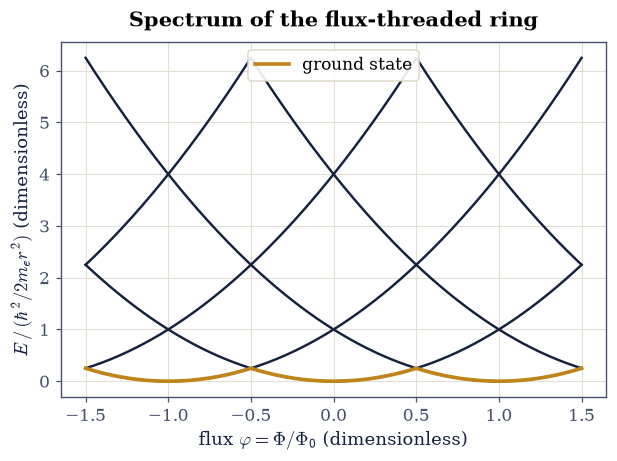
Fig. 607 Low-lying spectrum of a charged particle on a flux-threaded ring versus the dimensionless flux \(\varphi=\Phi/\Phi_0\), computed by exact diagonalization of the \(N=201\) Peierls ring. Each branch is one angular momentum \(m\), tracing the parabola \(E\propto(m-\varphi)^2\); the family repeats with period one (one flux quantum) and neighbouring branches cross at half-integer \(\varphi\), where the ground state changes its angular momentum.#
✓ exact diagonalization reproduces the Peierls ring's closed-form spectrum [max|Δ| = 2.88658e-15 (rtol=0, atol=1e-12)]
✓ the five lowest levels sit on the continuum parabolas (m - φ)² to the stated cos-series accuracy [max|Δ| = 2.22633e-06 (rtol=0.001, atol=1e-09)]
✓ one whole flux quantum is invisible: E(φ + 1) = E(φ) exactly [max|Δ| = 4.44089e-15 (rtol=0, atol=1e-12)]
True
Exercise 3 — The persistent current#
A flux-dependent energy is a current. In a ring at equilibrium the flux derivative of the energy is the circulating current,
the same thermodynamic-derivative move as pressure from \(-\partial E/\partial V\) in Volume V. For the ground state of the ring, Eq. 658 gives a current that is linear near \(\varphi = 0\), maximal approaching \(\varphi = 1/2\), and then jumps sign as the ground state hands over from \(m = 0\) to \(m = 1\): a sawtooth with the period of one flux quantum. This is a persistent current: it flows forever, in a normal (non-superconducting) ring, with no EMF driving it, exactly the phenomenon §3.7 could only name.
Part a) Compute the ground-state current in ring units (\(\Phi_0 = 1\)) at
\(\varphi = 0.2\) two ways: by a central difference of the numerical ground
energy, \(-[E_0(\varphi + \delta) - E_0(\varphi - \delta)]/2\delta\) with
\(\delta = 10^{-6}\) (each \(E_0\) from numpy.linalg.eigvalsh on your
Exercise 1 ring_hamiltonian), and
analytically, by differentiating the \(m = 0\) branch \(E_0 = 2t[1 -
\cos(2\pi\varphi/N)]\) of the closed-form spectrum:
\(I = -(4\pi t/N)\sin(2\pi\varphi/N)\). Verify the two agree to rtol=1e-6
(the central difference’s \(\delta^2\) error sits far below that).
Part b) Sweep \(\varphi \in [-1.5, 1.5]\) (301 points), computing the
ground-state current by the same central difference, and plot the sawtooth.
Verify the sign flip across \(\varphi = 1/2\): the current at \(\varphi = 0.45\)
is negative and the current at \(\varphi = 0.55\) is positive, equal in
magnitude to rtol=1e-9 by the symmetry \(E(\varphi) = E(-\varphi) =
E(1 - \varphi)\).
I(0.2): central diff -3.9086305139e-04 vs analytic -3.9086320067e-04
I(0.45) = -8.794186e-04, I(0.55) = 8.794192e-04
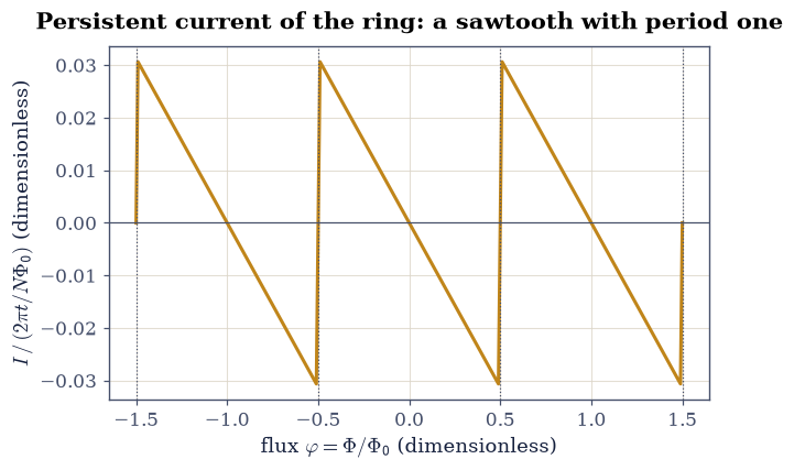
Fig. 608 Ground-state persistent current \(I=-\partial E_0/\partial\Phi\) of the \(N=201\) flux-threaded ring versus \(\varphi=\Phi/\Phi_0\), in ring units, computed by central differences of the exact ground energy. The current is a sawtooth with period one: linear response near integer flux, maximal approaching half-integer flux, and a sign jump at \(\varphi=1/2\) where the ground state’s angular momentum hands over from \(m=0\) to \(m=1\).#
✓ the persistent current: central difference of E₀ meets the analytic -(4πt/N) sin(2πφ/N) [got -0.000390863 vs expected -0.000390863 (rtol=1e-06, atol=1e-09)]
✓ the sawtooth jumps sign across φ = 1/2, where the ground state changes angular momentum [I(0.45) = -8.794e-04, I(0.55) = 8.794e-04]
✓ the jump is symmetric: E(φ) = E(1 - φ) forces I(0.55) = -I(0.45) [got 0.000879419 vs expected 0.000879419 (rtol=1e-09, atol=1e-09)]
True
Exercise 4 — The loop integral is topological#
Everything so far assumed that only the enclosed flux matters. This exercise computes it. An ideal solenoid of radius \(\rho_0\) on the \(z\)-axis, carrying total flux \(\Phi\), has (in the symmetric gauge of §3.6) the exterior vector potential
whose curl vanishes identically outside the solenoid (\(\mathbf B = 0\) where the particle travels), yet whose circulation \(\oint\mathbf A\cdot d\boldsymbol\ell\) around any loop enclosing the axis equals \(\Phi\) by Stokes’s theorem. The circulation cannot change under smooth deformations of the loop that avoid the solenoid: it counts the winding number around the flux, the topological heart of Eq. 657.
Fig. 609 shows the geometry: the flux region at the origin, and the three closed paths of Part b).
Part a) Implement Eq. 661 with \(\Phi = 1\) and verify with
loop_integral that the unit circle \(\bigl(\cos 2\pi s, \sin 2\pi s\bigr)\),
with its analytic tangent \(2\pi(-\sin 2\pi s, \cos 2\pi s)\), gives
\(\oint\mathbf A\cdot d\boldsymbol\ell = 1\) to rtol=1e-9: the trapezoid
rule in the parameter \(s\), fed the exact tangent, is spectrally accurate on
a smooth closed path, and 4001 points is already far past converged. (An
estimated tangent would cost six digits; the helper’s docstring says why.)
Part b) Deform without fear. Compute the same circulation, with
loop_integral and each path’s analytic tangent as in Part a), over (i) the
stretched-and-wobbled loop \(\bigl(2\cos 2\pi s,\; 1.2\sin 2\pi s + 0.3
\sin 6\pi s\bigr)\), still enclosing the origin once; (ii) the circle of
radius \(0.6\) centred at \((3, 0)\), \(\bigl(3 + 0.6\cos 2\pi s,\; 0.6\sin 2\pi
s\bigr)\), enclosing nothing; and (iii) the doubly-wound circle
\(\bigl(\cos 4\pi s, \sin 4\pi s\bigr)\). Expect \(\Phi\), \(0\), and \(2\Phi\): the
integral counts windings, and nothing else.
Part c) Add a gauge term and watch it drop out: with \(\chi(x, y) =
0.7\,x y\) (single-valued everywhere), verify that \(\mathbf A + \nabla\chi =
\mathbf A + 0.7\,(y,\, x)\) has the same circulation over the unit circle to
atol=1e-9. The gauge piece is a gradient; around any closed loop it
integrates to zero.
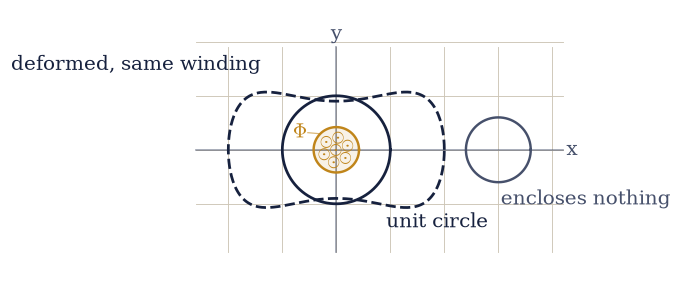
Fig. 609 Geometry of the circulation experiment: the flux region of an ideal solenoid (amber disk, field \(\mathbf B\) out of the page, total flux \(\Phi\)) seen end-on at the origin, with the three closed paths of the exercise. The unit circle and the deformed loop (ink) each wind once around the flux and share \(\oint\mathbf A\cdot d\boldsymbol\ell=\Phi\); the displaced circle at \((3,0)\) (grey) encloses no flux and has zero circulation.#
unit circle : 1.000000000000 (expect 1.0)
deformed loop : 1.000000000000 (expect 1.0)
outside loop : 0.00e+00 (expect 0)
double wind : 2.000000000000 (expect 2.0)
gauged : 1.000000000000 (expect 1.0)
✓ ∮A·dl over the unit circle equals the enclosed flux Φ (Stokes, spectrally-accurate trapezoid) [got 1 vs expected 1 (rtol=1e-09, atol=1e-09)]
✓ the circulation is topological: deformation leaves Φ, double winding gives 2Φ [max|Δ| = 0 (rtol=1e-06, atol=1e-09)]
✓ a loop that encloses no flux has zero circulation, however close it sits [got 0 vs expected 0 (rtol=1e-06, atol=1e-09)]
✓ adding ∇(0.7xy) moves A everywhere and the loop integral nowhere [got 1 vs expected 1 (rtol=1e-06, atol=1e-09)]
True
Exercise 5 — The shifted fringes#
Now the experiment itself. An electron leaves a source, passes a double slit, and lands on a screen; between the paths, behind the slits, sits the thin solenoid of Exercise 4 (Fig. 610). Each path acquires the phase \((q/\hbar)\int\mathbf A\cdot d\boldsymbol\ell\) along itself; the difference between the two paths is the closed-loop phase Eq. 657, \(2\pi\Phi/\Phi_0\), so the two-slit intensity becomes Eq. 659: the fringes translate rigidly by \(\Delta x = (\lambda L/d)(\Phi/\Phi_0)\), one full fringe spacing per flux quantum, while the electron never touches a field. Tonomura’s holography experiment [TOM+86] measured exactly this shift with the flux locked inside a shielded toroidal magnet: the phase difference across the torus was \(\pi\), half a fringe, because the enclosed flux was quantized at \(h/2e\) (Exercise 7 explains why that is the superconducting unit).
We use the parameters \(d = 1\), \(\lambda = 0.05\), \(L = 20\) (dimensionless model units), so the fringe spacing is \(\lambda L/d = 1\) exactly.
Part a) Write fringe_intensity(x, phi, d=1.0, lam=0.05, screen_l=20.0), returning Eq. 659 in units of the single-slit
intensity \(I_0\): \(4\cos^2(\pi d x/\lambda L + \pi\varphi)\), with x a
numpy array of screen positions and phi the enclosed flux in quanta.
Part b) With that fringe_intensity, evaluate \(I(x)\) on \(x \in [-3, 3]\)
(2001 points) for \(\Phi/\Phi_0 \in \{0, 1/4, 1/2\}\) and plot the three
patterns. Verify the two structural facts of Eq. 659: the
pattern at \(\Phi = \Phi_0\) equals the pattern at \(\Phi = 0\) pointwise
(atol=1e-12), and at \(\Phi = \Phi_0/2\) the central maximum has become an
exact zero, \(I(0) = 0\) (atol=1e-12): where fringes were brightest,
darkness, with no field touching the electron.
Part c) Measure the shift like an experimentalist: for
\(\Phi/\Phi_0 = 0.3\), locate the central fringe’s maximum by evaluating
\(I\) on a fine grid (\(10^5\) points on \([-1, 1]\)) and taking numpy.argmax,
then verify the measured peak position equals \(-0.3\) fringe spacings to
atol=1e-4 (the grid pitch; the sign says which way the fringes march:
toward the path with the lagging phase).
Part d) Animate the march: ramp \(\Phi\) from \(0\) to \(2\Phi_0\) over 80 frames and animate \(I(x)\) with a marker riding the central maximum. The validation checks the animated data: the marker’s trajectory across the ramp is the straight line \(x_{\max} = -(\Phi/\Phi_0)\) fringe spacings, wrapped to the central period.
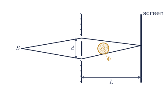
Fig. 610 The Aharonov–Bohm interferometer: electrons from the source \(S\) pass the double slit (separation \(d\)), and interfere on the screen at distance \(L\); the shaded amber disk between the paths is the end-on solenoid of flux \(\Phi\) (\(\mathbf B\) out of the page, zero along both paths). The two drawn paths enclose the flux, so their phase difference gains \(2\pi\Phi/\Phi_0\) on top of the geometric path difference.#
|I(Phi_0) - I(0)|_max : 4.44e-15
I(0) at half quantum : 1.50e-32
peak at phi = 0.3 : -0.30000 (expect -0.30000)
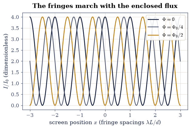
Fig. 611 Two-slit intensity \(I(x)/I_0=4\cos^2(\pi dx/\lambda L+\pi\Phi/\Phi_0)\) on the screen for enclosed flux \(\Phi=0\) (ink), \(\Phi_0/4\) (grey), and \(\Phi_0/2\) (amber), with slit separation \(d=1\), wavelength \(\lambda=0.05\), and screen distance \(L=20\), so the fringe spacing is \(\lambda L/d=1\). The pattern translates rigidly by \((\lambda L/d)\,\Phi/\Phi_0\); at half a flux quantum the central bright fringe has become an exact zero.#
Fig. 612 Animation of the two-slit intensity \(I(x)/I_0\) as the enclosed flux ramps linearly from \(0\) to \(2\Phi_0\): the fringes (ink) march rigidly leftward, one full spacing \(\lambda L/d\) per flux quantum, while the amber marker rides the central maximum. The pattern returns to itself at every integer \(\Phi/\Phi_0\); the electron crosses no field at any moment of the ramp.#
✓ one flux quantum restores the pattern pointwise: I(x; Φ₀) = I(x; 0) [max|Δ| = 4.44089e-15 (rtol=0, atol=1e-12)]
✓ at Φ = Φ₀/2 the central bright fringe is an exact zero [got 1.49976e-32 vs expected 0 (rtol=1e-06, atol=1e-12)]
✓ the measured peak position is -(Φ/Φ₀) fringe spacings: the predicted fringe shift, read off the screen [got -0.3 vs expected -0.3 (rtol=1e-06, atol=0.0001)]
✓ the animated marker's law holds across the ramp: the central maximum tracks x = -(Φ/Φ₀) within the central period [max|Δ| = 2.77556e-17 (rtol=1e-06, atol=0.0001)]
True
Exercise 6 — The scale of the effect#
How big is a flux quantum? For a single electron, Eq. 657 sets \(\Phi_0 = h/e\): two exactly-defined SI constants (both fixed by definition since 2019), so \(\Phi_0\) is exact. The striking part is how small it is, and therefore how accessible the effect: a micron-scale ring encloses one flux quantum in a field a refrigerator magnet would embarrass.
Part a) Compute \(\Phi_0 = h/e\) from scipy.constants (h and e)
and verify it equals \(4.135667696\times 10^{-15}\) Wb to rtol=1e-9
(the 2018 CODATA value is exact; the check pins the displayed digits).
Part b) For a ring of radius \(r = 1\ \mu\mathrm m\), compute the uniform
field that threads exactly one flux quantum through its area, \(B = \Phi_0 /
(\pi r^2)\), and verify \(B = 1.316\ \mathrm{mT}\) to rtol=1e-3: about
forty times the Earth’s field, trivially achievable, which is why
Aharonov–Bohm oscillations are a standard laboratory sight in mesoscopic
rings. Then compute the phase Tonomura’s toroid imprinted: an enclosed flux
of \(h/2e\) in Eq. 657 gives \(\Delta\varphi = \pi\) exactly, half a
fringe, the displacement his holograms show.
Phi_0 = h/e : 4.135667697e-15 Wb
B for one quantum : 1.3164 mT (r = 1 um)
Tonomura's phase : 1.000000000000 pi
✓ the electron's flux quantum h/e, from the exact SI h and e [got 4.13567e-15 vs expected 4.13567e-15 (rtol=1e-09, atol=1e-09)]
✓ one flux quantum through a 1 μm ring needs only B = 1.316 mT [got 0.00131642 vs expected 0.001316 (rtol=0.001, atol=1e-09)]
✓ an enclosed h/2e imprints a phase of exactly π: Tonomura's half fringe [got 3.14159 vs expected 3.14159 (rtol=1e-12, atol=1e-09)]
True
Exercise 7 — Flux quantization: a promise delivered#
§3.7 ended with a pointer this course could then only state: flux trapped in a superconducting ring comes in “discrete quanta \(h/2e\)”. The machinery of this notebook explains both the quantization and the puzzling factor of two.
In a superconductor the carriers condense into a single macroscopic wavefunction \(\Psi = \sqrt{n_s}\,e^{i\vartheta}\) (Volume VII builds the statistical mechanics behind such condensates). Deep inside the ring the current density vanishes, which pins the phase gradient to the vector potential: \(\hbar\nabla\vartheta = q\mathbf A\). Integrating around the ring and demanding \(\Psi\) be single-valued (\(\oint\nabla\vartheta\cdot d\boldsymbol\ell = 2\pi n\), \(n\in\mathbb Z\)) forces
The measured unit is \(h/2e\), not \(h/e\): the carriers have charge \(q = 2e\), because they are Cooper pairs. Flux quantization is therefore a charge-counting experiment, and it voted for pairing before the microscopic theory could explain it.
Part a) The pair charge halves the period, and the ring of Exercise 2
shows it directly. For charge \(q = 2e\) the link phases double,
\(\theta_j = 2\pi(2\varphi)/N\) with \(\varphi = \Phi/(h/e)\) still measured in
electron flux quanta. Verify with numpy.linalg.eigvalsh on your
Exercise 1 ring_hamiltonian that the full
spectrum at \(\varphi = 0.2\) equals the spectrum at \(\varphi = 0.7\)
(atol=1e-12): for pairs, the period in \(\Phi\) is \(h/2e\), half the
electron’s. Plot the two ground-state curves \(E_0(\varphi)\) for \(q = e\) and
\(q = 2e\) over \(\varphi\in[0, 1]\); the doubled charge traces two periods
where the single charge traces one.
Part b) Compute \(h/2e\) from scipy.constants and verify it against the
CODATA-listed magnetic flux quantum,
physical_constants["mag. flux quantum"] \(= 2.067833848\times10^{-15}\) Wb,
to rtol=1e-10: the constant the metrologists tabulate is the
superconducting unit, delivered here from first principles.
pair spectrum, phi=0.2 vs 0.7 : 2.66e-15
h/2e : 2.067833848e-15 Wb
CODATA tabulated: 2.067833848e-15 Wb
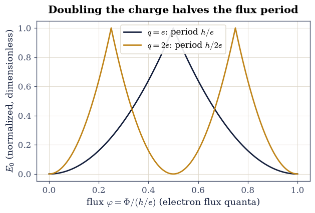
Fig. 613 Ground-state energy of the flux-threaded ring versus \(\varphi=\Phi/(h/e)\) for carrier charge \(q=e\) (ink) and \(q=2e\) (amber), from exact diagonalization of the \(N=201\) Peierls ring. Doubling the charge doubles every link phase, so the pair traces two full periods where the electron traces one: flux through a superconducting ring is pinned at multiples of \(h/2e\), the factor of two that identified Cooper pairing.#
✓ for charge-2e carriers the spectrum repeats after HALF an electron flux quantum: the pair's period is h/2e [max|Δ| = 2.66454e-15 (rtol=0, atol=1e-12)]
✓ h/2e equals the CODATA magnetic flux quantum: the discrete unit promised in §3.7, now derived [got 2.06783e-15 vs expected 2.06783e-15 (rtol=1e-10, atol=1e-09)]
True
Exercise 8 — The arc, closed (a reading exercise)#
No computation here; read this the way the Epilogue reads the course.
Track what the vector potential has been, volume by volume. In §3.6 it was a device: \(\mathbf B = \nabla\times\mathbf A\) made \(\nabla\cdot\mathbf B = 0\) automatic, and the gauge freedom looked like a defect to be managed. In §3.8 the freedom became a tool: the Lorenz gauge decoupled Maxwell’s equations into wave equations. In §3.12 it became structure: \(A^\mu\) assembled into a four-vector, and gauge invariance survived every boost. This notebook made it physics: the loop integral of \(\mathbf A\), the one gauge-proof thing it carries, moves interference fringes and pins the flux in superconducting rings, in regions where every field is zero.
The pattern, one more volume out, runs the other way: in quantum electrodynamics one starts from the local phase freedom Eq. 656 and derives the existence of \(\mathbf A\), of Maxwell’s equations, of the photon, as the price of making the symmetry local. Gauge invariance stops being a property of electromagnetism and becomes its origin, and the same logic (with grander symmetry groups) builds the rest of the Standard Model. That story is beyond this course; the Aharonov–Bohm effect is where it becomes impossible to dismiss.
One more horizon deserves its name. The phase Eq. 657 is the simplest example of a geometric phase: a phase acquired from the path traversed, not the time elapsed. Berry showed in 1984 [Ber84] that the same structure appears whenever a quantum system is carried slowly around a closed circuit in any parameter space, with the Aharonov–Bohm effect as the special case where the parameter is position around a flux. Berry phases now organize whole subjects (molecular dynamics near level crossings, the modern theory of polarization, topological band structure); the reader who wants the general machinery starts with his paper, carrying this notebook’s flux ring as the worked example.
Notebook summary#
A random per-site gauge transformation moved every link phase of the \(N = 201\) Peierls ring and no eigenvalue (agreement at \(10^{-12}\)), and was exactly the unitary \(U = \mathrm{diag}(e^{i\chi_j})\) of Eq. 656; winding the links by \(2\pi\cdot0.2/N\), by contrast, raised the enclosed flux from \(\varphi = 0.3\) to \(0.5\) and moved the ground state onto the \(\varphi = 0.5\) value. Only the loop sum is physical.
Exact diagonalization reproduced the ring’s closed-form spectrum to \(10^{-12}\) and the continuum parabolas \((\hbar^2/2m_e r^2)(m - \varphi)^2\) of Eq. 658 to the stated \(10^{-3}\); the spectrum was exactly periodic under \(\varphi \to \varphi + 1\).
The flux derivative Eq. 660 produced the persistent-current sawtooth: central differences met \(-(4\pi t/N)\sin(2\pi\varphi/N)\) to \(10^{-6}\), with the symmetric sign jump at half-integer flux.
The circulation \(\oint\mathbf A\cdot d\boldsymbol\ell\) of the solenoid potential Eq. 661 was \(\Phi\) on the unit circle and on a deformed loop, \(2\Phi\) on a double winding, \(0\) on a non-enclosing loop, and unmoved by the gauge term \(\nabla(0.7xy)\): a winding counter, to ten digits, by the trapezoid rule.
The two-slit pattern Eq. 659 marched by exactly \(-(\Phi/\Phi_0)\) fringe spacings (measured by peak location to \(10^{-4}\)), restored itself at one flux quantum, and zeroed its central fringe at half a quantum; Tonomura’s enclosed \(h/2e\) imprints exactly \(\pi\).
The scales: \(\Phi_0 = h/e = 4.135667696\times10^{-15}\) Wb exactly, one quantum through a 1 μm ring at \(B = 1.316\) mT; and for charge-\(2e\) carriers the ring’s period halved (spectra at \(\varphi = 0.2\) and \(0.7\) equal to \(10^{-12}\)), with \(h/2e\) matching the CODATA magnetic flux quantum to \(10^{-10}\): the §3.7 promise, delivered.
Outlook#
Berry phases [Ber84]. The flux ring is the archetype of a geometric phase; the general theory replaces “position around a solenoid” with any slow closed circuit in parameter space, and its curvature reappears in the anomalous velocity of Bloch electrons and the classification of topological bands.
Mesoscopic rings. In normal-metal rings below a micron, the \(h/e\)-periodic persistent current of Exercise 3 and Aharonov–Bohm conductance oscillations are routine measurements; disorder averages the \(h/e\) component and reveals an \(h/2e\) harmonic with a different origin (time-reversed path pairs) than the superconducting unit.
Superconducting quantization in the laboratory. SQUIDs count flux in units of \(h/2e\) and are the most sensitive magnetometers built; the same quantization underlies the fluxonium and flux qubits of the hardware §6.27 treated abstractly.
Local gauge symmetry as a construction principle. Demanding Eq. 656 locally generates electromagnetism; Volume VII’s Coda (§7.23) builds the many-body language in which that construction is written.
References#
Yakir Aharonov and David Bohm. Significance of electromagnetic potentials in the quantum theory. Physical Review, 115:485–491, 1959. doi:10.1103/PhysRev.115.485.
Michael V. Berry. Quantal phase factors accompanying adiabatic changes. Proceedings of the Royal Society of London A, 392:45–57, 1984. doi:10.1098/rspa.1984.0023.
David J. Griffiths and Darrell F. Schroeter. Introduction to Quantum Mechanics. Cambridge University Press, 3 edition, 2018.
John David Jackson. Classical Electrodynamics. Wiley, 3 edition, 1998.
Akira Tonomura, Nobuyuki Osakabe, Tsuyoshi Matsuda, Takeshi Kawasaki, Junji Endo, Shinichiro Yano, and Hiroji Yamada. Evidence for Aharonov–Bohm effect with magnetic field completely shielded from electron wave. Physical Review Letters, 56:792–795, 1986. doi:10.1103/PhysRevLett.56.792.