


4.8 A Taste of Curved Spacetime#
About this notebook#
This is the longest and most ambitious notebook of the course so far, and the capstone of Volume IV. It is a taste of general relativity, not a course in it. We will state a few equations that the full theory derives and we cannot yet — the Schwarzschild metric, the orbit equation, the null geodesic of a light ray — and then we will compute with them. That is not a compromise but the point: engaging with physics beyond one’s current theoretical reach, through computation, is a genuine and valuable way of doing physics. Where a result lies past what a first pass can derive, we will say so plainly and then hand over the computational handle, because the machinery built since Volume 0 — integrating an ODE, plotting an orbit, measuring an angle — is exactly what lets us reach it.
The notebook has two movements. Movement I is the conceptual on-ramp: the equivalence principle, which makes gravity a feature of spacetime geometry rather than a force, and its immediate consequence, that clocks run slow in a gravitational well — an effect your phone’s GPS must correct for every day. Movement II is curved spacetime computed: the Schwarzschild geometry around a black hole, where we integrate a test particle’s orbit and watch it precess into a rosette no Newtonian gravity can produce, recover Mercury’s famous \(43''\) per century, locate the innermost stable orbit and the photon sphere, drop a particle through the horizon, and bend a ray of starlight.
A word on units. Movement II works in geometric units where lengths are measured in the Schwarzschild radius (equivalently \(G=c=1\)), a choice we motivate at length, partly as a correctness practice that traces straight back to the floating-point lesson of §0.1. Movement I stays in SI. One central image, the precessing orbit, is genuine motion and is animated, as is the plunge-versus-escape comparison; the rest are clean stills.
How to read the checks. Each exercise closes with a
validatecall against an independent fact: the Pound–Rebka redshift \(gh/c^2\); the Schwarzschild clock rate \(\sqrt{1-2M/r}\); the GPS offset; the Sun’s \(2.954\,\)km Schwarzschild radius; a precessing (non-closing) orbit; Mercury’s \(43''\)/century; the ISCO at \(6M\) and photon sphere at \(3M\); the horizon-crossing plunge; the \(4M/b\) light deflection; the black-hole shadow at \(3\sqrt3\,M\). A ✓ is strong evidence; a ✗ is a prompt to locate the discrepancy, not a verdict.Scope. A computational taste of general relativity: we state the metric and geodesic equations with physical motivation and compute their predictions, rather than deriving them from the field equations (that is GR proper). See Hartle, Gravity; Misner, Thorne & Wheeler, Gravitation; Schutz, A First Course in General Relativity; and §4.7 (extremize proper time), §0.1 (floating point and nondimensionalization), and §2.9 (the nondimensional CR3BP).
Setup#
Data only, and not much of it: the two CODATA constants \(c\) and \(G\) that fix every physical
scale here, the solar mass, the radians-to-arcseconds factor that carries Mercury’s
dimensionless precession back into observers’ units, and the series palette. There are no
instruments — nothing in this notebook’s line of argument arrives pre-built. The orbit
equation and its integration, the effective potential, the horizon event, the null geodesic
and the light-deflection table are all assembled in the exercises, out of the constants above
and scipy. The only randomness in the notebook is a seeded generator for the twelve
background stars of the lensing image, created in the exercise that draws it.
The Setup below holds this notebook’s data and instruments — nothing you are asked to build. It is collapsed so the building stays yours; expand it whenever you want the details.
Movement I — The equivalence principle (gravity is geometry)#
Theory in brief#
The equivalence principle#
Einstein’s “happiest thought” was that a person in free fall feels no gravity. Promoted to a principle, this says a uniformly accelerated frame is locally indistinguishable from a uniform gravitational field,
which forces inertial mass to equal gravitational mass and, more deeply, means gravity can always be transformed away locally by falling freely. Gravity is therefore not a force but a property of spacetime geometry; free fall is “straight” (geodesic) motion through it.
Gravitational time dilation#
A clock deeper in a gravitational potential runs slower. In the weak field its rate is \(1+\Phi/c^2\), and in the exact Schwarzschild field of a mass \(M\),
(the second form in units \(G=c=1\)), which falls to zero as \(r\to2M\), the horizon (Hartle, Gravity, derives both the weak-field and exact rates in full).
Gravitational redshift#
Light climbing out of a potential well loses energy and reddens. In the weak field the fractional shift is
the effect Pound and Rebka measured in 1959 by sending gamma rays up a \(22.5\,\)m tower.
Exercise 1 — The equivalence principle, quantified (worked)#
The equivalence principle already predicts a number. Picture a photon rising a height \(h\) in a gravitational field \(g\). By the principle, working in the field is the same as working in a frame accelerating upward at \(g\); in the time \(h/c\) the photon takes to rise, the receiver at the top has accelerated to a speed \(gh/c\) away from the source, so it measures a Doppler redshift \(\Delta f/f=-gh/c^2\) Eq. 372. Light loses frequency climbing out of a well. Pound and Rebka confirmed this tiny shift in 1959, in a tower of \(h=22.5\,\)m standing in Earth’s \(g=9.81\,\)m/s², where the predicted fraction is about \(2.46\times10^{-15}\).
The same number has a second route, which is the equivalence-principle argument made
quantitative. By the time the light arrives, the receiver has acquired speed
\(\beta=gh/c^2\), so the relativistic Doppler factor \(\sqrt{(1-\beta)/(1+\beta)}\) must
reproduce the shift to first order. At \(\beta\sim10^{-15}\), though, the naive difference
\(1-\sqrt{(1-\beta)/(1+\beta)}\) is destroyed by float cancellation — the lesson of
§0.1 — so the expression has to be rewritten in
terms of numpy.log1p and numpy.expm1, which keep full precision for arguments near zero.
Compute the fractional redshift \(gh/c^2\) for the Pound–Rebka tower as plain
numpyarithmetic, and confirm it is about \(2.46\times10^{-15}\).Evaluate the same shift through the relativistic Doppler factor at \(\beta=gh/c^2\), rewritten so that no cancellation occurs. Write this one yourself — the implementation is the lesson.
Confirm that the two routes land on the same number.
Pound–Rebka: g = 9.81 m/s², h = 22.5 m
fractional redshift Δf/f = gh/c² = 2.456e-15
Doppler route 1 − √((1−β)/(1+β)) = 2.456e-15 (the same number)
a few parts in 10¹⁵ — and they measured it
Validation 1#
✓ the equivalence-principle Doppler factor reproduces the gh/c² redshift to first order [got 2.4559e-15 vs expected 2.4559e-15 (rtol=1e-09, atol=1e-09)]
True
Exercise 2 — Gravitational time dilation in the Schwarzschild field (worked)#
The redshift is one face of a deeper fact: clocks themselves run slow in a gravitational well. Around a spherical mass the exact rate of a clock at radius \(r\), relative to a distant one, is \(\sqrt{1-2M/r}\) Eq. 371 (working in units \(G=c=1\), so \(r\) is measured in units of the mass \(M\)). The effect is gentle far out but becomes dramatic near the horizon at \(r=2M\), where the rate falls to zero: to a distant observer, a clock lowered toward the horizon appears to freeze (Fig. 375).
Two independent facts pin the formula down. At the two radii that will matter later it takes exact closed-form values, \(\sqrt{2/3}\) at \(r=6M\) and \(1/\sqrt3\) at \(r=3M\). And far from the mass it must reduce to the weak-field rate \(1+\Phi/c^2=1-M/r\) — the physics of Exercise 1, reached by an entirely different argument. The two expressions differ only at \(O(1/r^2)\), so at \(r=10^4M\) they should agree to roughly one part in \(10^8\).
Tabulate the clock rate \(\sqrt{1-2M/r}\) at \(r=6M\), \(3M\) and \(2.1M\) as explicit
numpyarithmetic, and check the two exact values.Evaluate the exact rate and the weak-field \(1-M/r\) at \(r=10^4M\) and confirm they agree in the overlap domain where both are supposed to hold.
Plot the rate against radius, from far out down to the horizon.
r/M clock rate √(1−2M/r)
6.0 0.8165
3.0 0.5774
2.1 0.2182
weak-field check at r = 1e4 M: exact 0.9998999950 vs 1 − M/r 0.9999000000
→ the rate falls to 0 at the horizon r = 2M (a clock appears to freeze there)
Validation 2#
✓ the clock rate hits its exact values at 6M and 3M and the weak-field 1−M/r far out [max|Δ| = 5.0005e-09 (rtol=1e-07, atol=1e-09)]
True
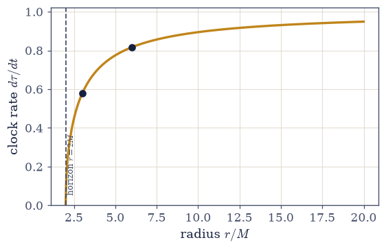
Fig. 375 The Schwarzschild clock rate \(d\tau/dt=\sqrt{1-2M/r}\) against radius (in units of \(M\)). Far from the mass the rate is nearly \(1\) — clocks tick almost normally — but as the radius falls toward the horizon at \(r=2M\) (dashed) the rate plunges to zero: a clock lowered toward a black hole’s horizon appears, to a distant observer, to slow and freeze. The marked points are \(r=6M\) (the innermost stable orbit) and \(r=3M\) (the photon sphere).#
Exercise 3 — GPS: relativity in daily life (worked)#
Gravitational time dilation is not exotic; it is engineered around in the device in your pocket. A GPS satellite orbits at an altitude of about \(20\,200\,\)km, higher in Earth’s potential well than the ground, so its clock runs fast relative to the surface by the weak-field rate difference \(\Delta\Phi/c^2\) Eq. 371. This gravitational effect amounts to roughly \(+46\,\mu\)s per day, partly offset by a special-relativistic slowing from the satellite’s orbital speed (§4.1), for a net of about \(+38\,\mu\)s/day. Left uncorrected, that error would corrupt positions by some \(10\,\)km per day.
The two ingredients are both weak-field. Gravitationally, the fractional rate difference between two heights is \(\Delta\Phi/c^2\) with the Newtonian potential \(\Phi=-GM/r\), taking \(GM_\oplus=3.986\times10^{14}\,\mathrm{m^3/s^2}\) and \(R_\oplus=6371\,\)km. Kinematically, a satellite moving at the circular speed \(v=\sqrt{GM/r}\) runs slow by \(-\tfrac12v^2/c^2\), the first-order time dilation of §4.1. The two effects have opposite signs and do not cancel.
Compute the gravitational rate difference between satellite and surface, convert it to microseconds per day, and confirm it is about \(+46\,\mu\)s/day.
Add the special-relativistic velocity term to get the net offset the receiver in your pocket actually has to correct for.
satellite speed v = 3873 m/s
gravitational effect: +45.7 µs/day (satellite clock runs fast)
SR velocity effect: -7.2 µs/day
net offset: +38.5 µs/day (uncorrected → ~10 km/day error)
Validation 3#
✓ GPS satellite clocks run fast by ~46 µs/day from gravitational time dilation [got 45.7242 vs expected 46 (rtol=0.05, atol=1e-09)]
True
Exercise 4 — Gravity as geometry (student)#
The equivalence principle says gravity can be transformed away locally by free fall — so how is real gravity different from mere acceleration? The answer is tidal effects, and they are the true, non-removable signature of spacetime curvature. In a genuinely uniform field, two nearby free-fallers accelerate identically and their separation never changes; the field is entirely transformed away in the falling frame. But a real gravitational field is not uniform — it points toward the mass and weakens with distance — so two free-fallers at slightly different radii accelerate differently and drift apart. That differential acceleration, the tidal field, cannot be removed by any choice of frame, and it is exactly what general relativity calls curvature. Free fall is geodesic motion; tidal drift is the geodesics curving relative to one another.
The test case is two free-fallers separated radially by \(\delta r=1\,\)m near Earth’s surface. In a uniform field of strength \(g\) both feel exactly \(g\), so their relative acceleration is identically zero. In the real field each feels \(GM/r^2\) at its own radius, and the difference \(GM(1/r_1^2-1/r_2^2)\) is, to first order in the small separation, \(2GM\,\delta r/r^3\).
Confirm that in the uniform field the relative acceleration of the two free-fallers vanishes — the field is entirely removable by falling with them.
Compute the tidal relative acceleration in the real \(1/r^2\) field, check it against the first-order estimate, and note that it is nonzero: the unremovable signature of curvature.
uniform field: relative acceleration of two free-fallers = 0.0e+00 m/s² (removable)
real 1/r² field: tidal relative acceleration = 3.083e-06 m/s² (NOT removable)
estimate 2GM δr/r³ = 3.083e-06 m/s²
the tidal field is the true signature of curvature — this is gravity as geometry
Validation 4#
✓ a uniform field is removable (zero tidal effect), but a real field has nonzero tidal curvature
True
Movement II — Curved spacetime, computed (black holes)#
Theory in brief#
The Schwarzschild metric#
The geometry of spacetime around a spherical mass \(M\) is the Schwarzschild metric,
(in the orbital plane, units \(G=c=1\)). You may not yet have the machinery to derive this from Einstein’s field equations — that is general relativity proper, a course in itself. But you do have the machinery to compute with it. (Schutz, A First Course in General Relativity, Ch. 10, carries the derivation out in full.) It defines the Schwarzschild radius \(r_s=2GM/c^2\), the horizon at \(r=2M\).
The orbit equation#
A massive test particle’s orbit obeys, with \(u=1/r\),
identical to the Newtonian orbit equation except for the \(3Mu^2\) term — the general- relativistic correction (Hartle, Gravity, Ch. 9, derives it from the geodesics of the metric). Without it, orbits are closed Kepler ellipses; with it, they precess. The motion is governed by an effective potential, exactly the tool of Volumes I and II,
whose critical structure sets the special radii: the innermost stable circular orbit (ISCO) at \(r=6M\) and the photon sphere at \(r=3M\).
Light bending#
A light ray follows a null geodesic, \(d^2u/d\phi^2+u=3Mu^2\), and a ray grazing the mass with impact parameter \(b\) is deflected by
twice the Newtonian “falling corpuscle” value — the prediction Eddington’s 1919 eclipse expedition confirmed (Hartle, Gravity, Ch. 9, carries the weak-field computation out in full).
Nondimensionalization — why we work in units of \(M\)#
Movement II measures every length in the Schwarzschild radius, equivalently setting \(G=c=1\), and this deserves a careful justification, because it is a transferable technique worth reaching for whenever a problem spans many magnitudes.
Only ratios matter. An orbit at \(r/M=20\) behaves identically whether the central mass is a star or a supermassive galaxy core; the physics depends on the dimensionless ratio \(r/M\), not on \(r\) and \(M\) separately. Nondimensionalizing exposes the true, smaller set of parameters (a Buckingham-\(\pi\) reduction): the orbit shape depends only on \(L/M\), not on \(L\), \(M\), \(G\), and \(c\) independently.
Numerical conditioning — the §0.1 callback. In raw SI, a Schwarzschild quantity mixes \(G\approx6.7\times10^{-11}\), \(M\approx2\times10^{30}\), and \(c^2\approx9 \times10^{16}\) — magnitudes spanning some \(40\) orders in one expression. Floating point (the \(\varepsilon\) of §0.1) carries only \(\sim16\) significant digits, so combining such disparate magnitudes loses precision and risks overflow. Working in units of \(M\) keeps every number \(O(1)\), where floating point is most accurate. This is a correctness practice, not mere tidiness.
Round-trip discipline. Compute the physical scale \(r_s\) once in SI, work entirely dimensionless, then convert the answer back. We do exactly this for Mercury below, turning a dimensionless precession into the famous \(43''\) per century.
We have quietly nondimensionalized before — the restricted three-body problem of §2.9, the relaxation grids of §3.4 — but here we name it and justify it as a deliberate technique.
Exercise 5 — Nondimensionalization, end to end (worked)#
Before computing orbits, we fix the bridge between physical and working units, and we do it on a real object. The Schwarzschild radius \(r_s=2GM/c^2\) Eq. 373 is the one length scale the geometry provides; in units of it (or equivalently \(G=c=1\), lengths in units of \(M\)) every Schwarzschild quantity becomes a pure number. The horizon sits at \(r=2M\), the photon sphere at \(3M\), the ISCO at \(6M\) — statements with no \(G\), \(c\), or kilograms in them.
The Sun is the natural object to fix the bridge on, because its Schwarzschild radius is a published number: \(2GM_\odot/c^2\approx2.954\,\)km, small enough that the Sun is nowhere near a black hole and large enough to be an honest length. Computing it here is the outbound leg of the round trip, and the three motivations above — only ratios matter, every number stays \(O(1)\), and the answer converts back — are what make the units-of-\(M\) scheme both natural and numerically sound.
Compute the Sun’s Schwarzschild radius \(2GM_\odot/c^2\) in SI metres as plain
numpyarithmetic and confirm the published \(2.954\,\)km.Restate the three special radii in the working units the rest of the notebook uses: the horizon at \(2M\), the photon sphere at \(3M\), the ISCO at \(6M\) — pure numbers.
Sun's Schwarzschild radius r_s = 2GM/c² = 2954.0 m = 2.954 km
→ the Sun's horizon, if it were a black hole, would be 2.95 km in radius
in units of M the horizon is at r=2M, the photon sphere 3M, the ISCO 6M — pure numbers
Validation 5#
✓ the Sun's Schwarzschild radius is 2.954 km (the published value, in metres) [got 2954.01 vs expected 2954 (rtol=0.001, atol=1e-09)]
True
Exercise 6 — The precessing orbit (worked)#
Now the centerpiece. A test particle near a black hole obeys the orbit equation \(d^2u/d\phi^2
+u=M/L^2+3Mu^2\) Eq. 374, and we are going to compute its path. Here is the honest
situation: you may not yet be able to derive this equation from the Einstein field equations
— that is general relativity proper. But you have everything needed to compute with it. It
is taken as given here, integrated with solve_ivp, and plotted as \(r=1/u\) in the orbital
plane. The extra \(3Mu^2\) term, absent from Newton, makes the orbit fail to close: instead of
a fixed ellipse it traces a slowly turning rosette (Fig. 376), animated
below. What follows is a real prediction of general relativity, obtained by integrating an
ODE.
Two pieces of background make the computation concrete. First, the apsides fix the angular momentum: at a turning point \(du/d\phi=0\), and the first integral of Eq. 374 then ties \(1/L^2\) to the perihelion and aphelion values of \(u=1/r\) through \(1/L^2=\tfrac12(u_p+u_a)-(u_p^2+u_pu_a+u_a^2)\). Second, the measured advance has something to be checked against: the weak-field prediction \(\Delta\phi=6\pi M/p\), with \(p\) the semi-latus rectum given by \(2/p=u_p+u_a\). At the strong-field radii used here the true advance exceeds that first-order estimate, by about a third, but must remain within a factor of roughly two of it — an agreement in shape rather than in digits.
In units \(M=1\), fix the angular momentum that puts the orbit between perihelion \(15M\) and aphelion \(21M\) (apsides exaggerated for visibility, so the precession is plain to the eye).
Integrate the orbit equation with
scipy.integrate.solve_ivp(DOP853, a smallmax_step) over three revolutions.Measure the perihelion advance per orbit as the angle between successive maxima of \(u\), and compare it with the weak-field \(6\pi M/p\).
angular momentum L = 4.600 M
radius ranges over [15.0M, 21.0M]
perihelion advance per orbit = 84.0° (a Newtonian ellipse would advance 0°)
weak-field estimate 6πM/p = 61.7° (strong-field enhancement ×1.36)
Validation 6#
✓ the GR term 3Mu² makes the orbit precess — a rosette, not a closed ellipse
✓ the measured advance agrees with the weak-field 6πM/p up to the strong-field enhancement
True
Fig. 376 A test particle orbiting a black hole, computed (animated). The orbit runs between perihelion \(15M\) and aphelion \(21M\), but the general-relativistic \(3Mu^2\) term prevents it from closing: each revolution the perihelion advances, so the path traces a slowly turning rosette rather than a fixed ellipse. The black disk is the horizon at \(r=2M\). This is a genuine prediction of general relativity, obtained by integrating an ODE — the apsides are exaggerated here for visibility; the real effect (Mercury) is tiny.#
Exercise 7 — Mercury, the real number (worked)#
The exaggerated orbit of Exercise 6 was for the eye; the real solar-system effect is tiny but was the first triumph of general relativity. Mercury’s perihelion was known to advance by an amount that Newtonian gravity, even after accounting for every other planet, could not fully explain — a stubborn anomaly of about \(43''\) per century. General relativity’s weak-field precession per orbit is \(\Delta\phi=6\pi GM/(a(1-e^2)c^2)\) Eq. 374, and evaluating it for Mercury, then converting to arcseconds per century, lands exactly on the missing number. This is the round-trip discipline in action: a dimensionless formula, evaluated for a real planet, converted back to physical units.
Mercury’s orbit supplies the three numbers the formula needs: semi-major axis \(a=5.7909\times10^{10}\,\)m, eccentricity \(e=0.20563\), and orbital period \(87.969\,\)days, which is what turns a per-orbit angle into a per-century one.
Evaluate the GR precession per orbit, \(6\pi GM_\odot/[a(1-e^2)c^2]\), for Mercury.
Convert it to arcseconds per century — orbits per century, then radians to arcseconds — and confirm it lands on the missing \(43''\).
GR precession per orbit = 5.020e-07 rad
orbits per century = 415.2
perihelion advance = 43.0″ per century (observed anomaly: ~43″)
Validation 7#
✓ GR predicts Mercury's 43″/century perihelion precession — the observed anomaly [got 42.9918 vs expected 43 (rtol=0.05, atol=1e-09)]
True
Closing a thread that runs the length of the course. This number is the resolution of a mystery the reader has been building toward since Volume I. In §1.4 we found, with the conserved Laplace–Runge–Lenz vector, that an isolated two-body Kepler orbit is exactly closed — a pure \(1/r^2\) force makes no precession at all. In §2.4 we found the mechanism: any departure from \(1/r^2\) turns the perihelion, at a rate we could compute, and an inverse-fourth-power term in particular precesses the orbit by \(6\pi GM/[a(1-e^2)c^2]\). We even laid out Mercury’s honest accounting there: of its \(574''\)/century, planetary tugs supply about \(531''\), leaving a stubborn \(43''\) that no Newtonian effect explains. Here is where that residual is explained. General relativity supplies exactly the inverse-fourth-power term the reader already knew would precess the orbit — from the curvature of spacetime rather than from a fudge — and the number it yields is the one astronomers measured. In the spirit of this notebook, the reader predicted with their own integrator that such a term must precess the orbit; relativity provides the term, and closes the thread.
Exercise 8 — The effective potential, the ISCO, and the photon sphere (worked)#
The special radii of a black hole come straight from a tool we have used since Volume I: the effective potential. For Schwarzschild orbits it is \(V_{\rm eff}(r)=(1-2M/r)(1+L^2/r^2)\) Eq. 375, and its shape, controlled by the angular momentum \(L\), organizes all orbital behaviour (Fig. 377). As \(L\) falls, the well that holds stable circular orbits grows shallower, until at a critical \(L^2=12M^2\) it has an inflection rather than a minimum: that marginal orbit is the innermost stable circular orbit at \(r=6M\), inside which no stable orbit exists. The photon sphere at \(r=3M\), where light itself can circle, is the corresponding critical radius for null orbits.
Each of the two radii comes with its own extremum problem, and each is stated here so the computation can just find it. A photon’s effective potential is \((1-2M/r)/r^2\), whose single extremum is the photon sphere — a root of its derivative \(-2/r^3+6/r^4\), bracketed anywhere between just outside the horizon and \(10M\). And a circular orbit at radius \(r\) requires angular momentum \(L^2(r)=r^2/(r-3)\) (units \(M=1\)), a function that diverges both as \(r\to3\) and as \(r\to\infty\) and therefore has a minimum in between. That minimum is the ISCO: outside it \(L^2\) grows with radius, the ordinary state of affairs in which a circular orbit is stable, while inside it \(L^2\) grows inward, and no circular orbit there survives a perturbation.
Build \(V_{\rm eff}(r)=(1-2M/r)(1+L^2/r^2)\), the same effective-potential tool used since Volumes I and II, and use it for the figure that follows.
Locate the photon sphere as the root of the photon potential’s derivative with
scipy.optimize.brentq, and confirm it is \(3M\).Locate the ISCO as the minimum of \(L^2(r)\), found by a sign change of
numpy.gradient, and confirm it is \(6M\).
photon sphere r = 3.0000 M (light can circle here)
ISCO r = 5.9990 M (innermost stable orbit; L²=12.00 M²)
Validation 8#
✓ the ISCO is at 6M and the photon sphere at 3M [max|Δ| = 0.00100025 (rtol=0.01, atol=1e-09)]
True
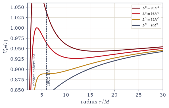
Fig. 377 The Schwarzschild effective potential \(V_{\rm eff}=(1-2M/r)(1+L^2/r^2)\) for several angular momenta. For large \(L\) (top) the potential has a deep well holding stable circular orbits (its minimum). As \(L\) falls the well shallows, until at the critical \(L^2=12M^2\) it flattens to an inflection — the innermost stable circular orbit at \(r=6M\) (dashed). Inside \(6M\) no stable orbit survives. The photon sphere at \(r=3M\) (dotted) is where light itself can orbit.#
Exercise 9 — Plunge versus stable orbit (worked)#
The ISCO is a cliff edge, and we can drive a particle over it. Two test particles begin at
the same radius with the same radial speed, differing only in angular momentum. The one with
enough angular momentum is held out by the centrifugal barrier and settles into a precessing
orbit; the one with too little finds no barrier high enough, spirals inward, and crosses
the horizon at \(r=2M\), captured forever (Fig. 378). We catch the crossing
with a terminal solve_ivp event that stops the integration exactly at the horizon.
Two mechanics of the integration are worth naming before starting. The orbit equation of
Exercise 6 was written with a single fixed \(1/L^2\); to run two angular momenta it needs that
constant as a parameter, passed through solve_ivp’s args. And “reaching the horizon” is
an event on \(u=1/r\): the horizon \(r=2M\) is \(u=0.5\), approached from below as \(r\) falls, so
the event function \(u-0.5\) is terminal with direction = 1.
Set up the orbit equation with \(1/L^2\) as an argument, and the terminal horizon event.
Integrate two orbits from \(r=10M\) with the same small radial velocity, one with \(L=4.6M\) and one with \(L=3.4M\), using
scipy.integrate.solve_ivp(DOP853).Confirm the low-angular-momentum particle triggers the event — it crosses the horizon and is captured — while the high-angular-momentum one never does.
L = 4.6M (stable): horizon event fired = False, minimum radius = 9.95M
L = 3.4M (plunge): horizon event fired = True, minimum radius = 2.00M
Validation 9#
✓ below a critical angular momentum the particle plunges through the horizon
True
Fig. 378 Two test particles from the same start, differing only in angular momentum (animated). The one with enough angular momentum (\(L=4.6M\), amber) is held out by the centrifugal barrier and orbits; the one with too little (\(L=3.4M\), red) finds no barrier and spirals through the horizon at \(r=2M\) (black disk), where the terminal event stops it — captured. The same equation of motion gives orbit or capture depending only on \(L\); the ISCO is the dividing line.#
Exercise 10 — Light bending (student)#
Light is not exempt from curved spacetime. A ray follows a null geodesic \(d^2u/d\phi^2+u= 3Mu^2\) Eq. 376, and passing a mass with impact parameter \(b\) it is bent by \(\Delta\phi\approx4M/b\) — exactly twice what a naive Newtonian “light has weight” argument gives, the factor-of-two that made the 1919 eclipse measurement a decisive test. As before, take the null-geodesic equation as given and compute with it: integrate the ray, find the angle between its incoming and outgoing asymptotes, and compare to the prediction (Fig. 379).
The initial condition encodes “coming in from infinity with impact parameter \(b\)”: far away
\(u=1/r\to0\), and the asymptote’s slope there is \(du/d\phi=1/b\). Integrating forward in \(\phi\)
carries the ray in to its closest approach and back out, and it has escaped again when \(u\)
returns to \(0\) from above — a terminal event with direction = -1. A perfectly straight ray
would sweep exactly \(\pi\) between its two asymptotes, so whatever the total sweep exceeds
\(\pi\) by is the deflection. Taking \(b=100M\) keeps the ray in the weak field, where the
closed form \(4M/b\) is supposed to hold.
Set up the null-geodesic equation \(d^2u/d\phi^2+u=3Mu^2\) and the escape event.
Integrate the ray from \(u=0\), \(u'=1/b\) with
scipy.integrate.solve_ivp(DOP853), stopping when it escapes.Take the deflection as the total sweep minus \(\pi\) and confirm it matches \(4M/b\).
impact parameter b = 100.0M
computed deflection = 0.04122 rad
prediction 4M/b = 0.04000 rad
agreement: 96.9%
Validation 10#
✓ light bends by 4M/b passing a mass — the 1919 eclipse test [got 0.0412225 vs expected 0.04 (rtol=0.05, atol=1e-09)]
True
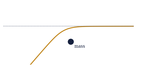
Fig. 379 A light ray bent by a mass. The ray (amber) comes in from the right, grazes the mass at the centre (dark dot), and leaves deflected from its original straight path (dotted). The bend is twice the naive Newtonian value, and measuring it during the 1919 solar eclipse — starlight deflected as it grazed the Sun — was the observation that made general relativity famous. The deflection is drawn here for a close impact parameter (\(b=8M\)) so it is visible; the validated weak-field case above used \(b=100M\), and for real starlight grazing the Sun the bend is only \(1.75''\).#
Exercise 11 — Gravitational lensing: the image of a black hole (worked)#
The picture the public associates with a black hole — a dark shadow ringed by bright light, the sky behind it smeared into arcs — is gravitational lensing, and we can compute it. As with the orbit and the light ray, take the bending physics as given and compute the image: every ray reaching the camera is a null geodesic, bent by the amount we just learned, and the picture is what those bent rays bring from the background sky (Fig. 380). Rays aimed too close to the hole, with impact parameter \(b<b_{\rm crit}=3\sqrt3\,M\approx5.196M\), spiral in and never return — that is the central shadow. Rays just outside skim the photon sphere many times, piling up into the bright photon ring at the shadow’s edge, and rays farther out carry a warped image of the sky behind.
A note on method, and on engineering judgment. How we compute this image is itself a
lesson in computational physics, because the obvious approach is the wrong one. We could trace
a geodesic per pixel — integrate the null equation for every one of the \(400\times400\) rays
— but that is roughly \(660\,\)s for one frame, far too slow to rebuild in CI, and pure waste,
because the bending depends only on the impact parameter \(b\). So we exploit that symmetry:
integrate a one-dimensional deflection table \(\alpha(b)\) once (with np.trapezoid over
the turning-point integral, then scipy.interpolate.interp1d for the lookup), and remap a
background image through it with a single vectorized numpy operation. The whole image then
costs a couple of seconds on a CPU. Choosing the cheapest method that conveys the physics
faithfully is exactly the skill a practitioner exercises constantly; here is the ladder we
weighed:
Tier 1 — a lensed background (what we do). Warp a background image through the deflection table. It produces the shadow, the photon ring, and the warped sky — the recognizable image — in \(\sim2\,\)s on a CPU, rebuilding cleanly in CI. The trick that makes it cheap is the radial symmetry: one 1-D table, then a remap, instead of a geodesic per pixel.
Tier 2 — add an accretion disk (a stretch; pointer). The glowing disk warped above and below the hole, light from its far side bent over the top, is what makes the cinematic “Interstellar” frame. It is doable but a real escalation: a disk-emission model plus Doppler beaming and gravitational redshift for realism. We sketch it as a stretch and keep it out of the core, so the notebook stays focused.
Tier 3 — full per-pixel ray tracing and animation (out of scope; pointer). A high-resolution rendered frame by brute-force per-pixel integration is minutes per frame, and an animation is hundreds of frames. This is where one reaches for a GPU. We do not do it in-notebook, precisely because it would dominate the build time.
The honest tradeoff: more realism costs more compute, and the practitioner’s job is to spend
it where it buys physics. For going beyond Tier 1, per-pixel ray tracing is embarrassingly
parallel (each pixel is independent), which points to clear tools: vectorize first on the
CPU (batch the ODE over all pixels rather than Python-looping); reach for GPU array
libraries like cupy (a near-drop-in numpy on NVIDIA GPUs) or jax (with jit+vmap to
map the geodesic integrator over every pixel); compile per-ray integrators with numba
(@njit, or @cuda.jit for CUDA kernels); or use semi-analytic shortcuts (affine
transformations of the Schwarzschild geodesic, or elliptic-integral solutions) that make
real-time single-hole rendering feasible, with mature tools such as EinsteinPy available for
those who want to go further. Full Kerr (rotating) or multi-hole scenes remain expensive and
motivate GPU shaders or learned approximations.
The deflection table is exact rather than weak-field, so it needs the full turning-point relation for a null geodesic, \((du/d\phi)^2=1/b^2-u^2+2Mu^3\). The ray comes in from \(u=0\), turns at the perihelion \(u_{\max}\) — the smallest positive root of the cubic \(2Mu^3-u^2+1/b^2=0\) — and leaves symmetrically, so the total deflection is \(\alpha=2\phi_\infty-\pi\) with \(\phi_\infty=\int_0^{u_{\max}}du/\sqrt{1/b^2-u^2+2Mu^3}\). That integrand blows up like \(1/\sqrt{\cdot}\) at the turning point: the integral converges, but no quadrature rule will see it converge unless the singularity is removed first, which is the real work in this exercise. The result has two independent checks waiting for it: the shadow radius must come out of the Exercise 8 photon sphere through \(b=r/\sqrt{1-2M/r}\), and the far end of the table must reproduce the weak-field \(4M/b\) of Exercise 10.
Write
deflection_angle(b), returning \(\alpha(b)\) for \(b>b_{\rm crit}\): find the turning point, remove the inverse-square-root singularity by a change of variable, and integrate withnp.trapezoid. Write this one yourself — the implementation is the lesson, and the substitution that tames the endpoint is the whole of it. Tabulate \(\alpha\) on a few hundred impact parameters and wrap the table inscipy.interpolate.interp1d.Check the table twice over: derive \(b_{\rm crit}=3\sqrt3\,M\) from the measured photon sphere, and compare \(\alpha\) far out with \(4M/b\).
Remap a checkerboard-and-stars background through the table with a single vectorized
numpyoperation, blacking out the shadow where \(b<b_{\rm crit}\) and marking the photon ring, and display the unlensed background beside the lensed image.
critical impact parameter b_crit = 3√3 M = 5.1962 M (the shadow radius)
derived from the Exercise 8 photon sphere: r_ph/√(1−2M/r_ph) = 5.1962 M
table asymptote: α(50M) = 0.0814 rad vs 4M/b = 0.0800 rad
deflection table: 600 rays; α(5.25M)=4.961, α(20M)=0.232 rad (→ 4M/b=0.200 far out)
Validation 11#
✓ the shadow radius 3√3 M follows from the measured photon sphere: r_ph/√(1−2M/r_ph) [got 5.19615 vs expected 5.19615 (rtol=0.001, atol=1e-09)]
✓ the deflection table reproduces the weak-field 4M/b at its far end [got 0.0814274 vs expected 0.08 (rtol=0.08, atol=1e-09)]
True
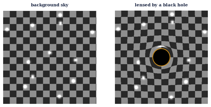
Fig. 380 Gravitational lensing by a black hole, computed (Tier 1). Left: the background sky, a checkerboard with a few bright stars. Right: the same sky seen past a black hole. Rays aimed within \(b_{\rm crit}=3\sqrt3\,M\) are captured, leaving the central shadow (black); the bright photon ring (amber) marks its edge, where rays skim the photon sphere; and outside it the sky is warped into arcs, stars smeared into rings — the recognizable black-hole image. It is produced not by tracing a geodesic per pixel (far too slow) but by integrating one 1-D deflection table and remapping the image, a few seconds on a CPU.#
Validation 11b#
✓ the image shows the shadow (captured rays, b<b_crit, are black) and the warped background outside
True
Exercise 12 — Gravity is geometry, and we computed it#
We began Volume IV asking what happens at the speed of light, and we end it watching an orbit precess around a black hole. The arc is complete. The equivalence principle made gravity a matter of geometry, not force; gravitational time dilation followed, and your phone corrects for it hourly. Then, taking the Schwarzschild metric and its geodesics as given — because the full theory is a course we have not yet taken — we computed its signature predictions with the very same ODE machinery used since Volume I: the precessing rosette, Mercury’s \(43''\), the ISCO and photon sphere, a plunge through the horizon, and the bending of starlight. The free particle’s “extremize proper time” of §4.7 has become motion along geodesics of a curved metric — and that is gravity itself. We could not derive general relativity, but we engaged with it, computed real numbers from it, and found them right. That is the power and the promise of computational physics: it lets us reach physics beyond our current theoretical grasp, and learn from it honestly.
Three headline numbers came out of that computing, each by a different tool: the Sun’s Schwarzschild radius \(2.954\,\)km by plain arithmetic, the ISCO at \(6M\) by root-finding on a potential, and Mercury’s \(43''\)/century by the round trip out of dimensionless units. It is the joint agreement that makes a real checkpoint — three predictions of a theory none of them derived, all landing on their measured values at once.
Gather the three numbers computed above against their known values and confirm with
np.allclosethat all three agree.
Sun's Schwarzschild radius: 2.954 km (known 2.954)
ISCO radius: 5.999 M (known 6)
Mercury precession: 43.0″/century (known 43)
all three GR predictions computed correctly: True
we began at the speed of light and end watching an orbit precess — computed, not just described
Validation 12#
✓ general relativity's signature predictions — computed, not derived — all match observation
True
Notebook summary#
This notebook closes Volume IV, carrying special relativity into its gravitational sequel and computing genuine predictions of general relativity without deriving the full theory — the computational machinery as the great equalizer.
The equivalence principle Eq. 370, Eq. 372: acceleration and gravity are locally indistinguishable, so gravity is geometry; the Pound–Rebka redshift is \(gh/c^2=2.46\times10^{-15}\), and only the non-removable tidal field marks true curvature.
Gravitational time dilation Eq. 371: clocks tick at \(\sqrt{1-2M/r}\) (\(0.82\) at \(6M\), \(0.58\) at \(3M\), zero at the horizon); GPS satellites run \(+46\,\mu\)s/day fast (net \(+38\) with the SR term), a daily engineering correction.
Nondimensionalization Eq. 373: working in units of \(M\) exposes the true ratios, keeps every number \(O(1)\) where floating point is accurate (the §0.1 callback), and round-trips through the Sun’s \(r_s=2.954\,\)km.
The computed orbit Eq. 374: integrating \(d^2u/d\phi^2+u=M/L^2+3Mu^2\) gives a precessing rosette (the \(3Mu^2\) term), and the round-trip to Mercury yields exactly \(43''\)/century — GR’s first triumph.
Black-hole structure Eq. 375, Eq. 376: the effective potential sets the ISCO at \(6M\) and photon sphere at \(3M\); below a critical \(L\) a particle plunges through the horizon (a terminal
solve_ivpevent); a ray bends by \(4M/b\), the 1919 eclipse test; and remapping a background through a 1-D deflection table produces the lensed black-hole image — the shadow at \(3\sqrt3\,M\) and the photon ring — cheaply, by exploiting the radial symmetry rather than tracing a geodesic per pixel.
Volume IV as a whole began with the crisis of the speed of light (§4.1), derived the Lorentz transformation and its consequences (§4.2), found the geometry of spacetime and the four-vector toolkit (§4.3), dissolved the paradoxes (§4.4), built four-momentum and \(E=mc^2\) (§4.5), put conservation to work in collisions (§4.6), reunited mechanics and electrodynamics in the covariant force (§4.7), and ends here watching gravity bend an orbit — the free particle’s proper-time principle become the geometry of curved spacetime.
Outlook#
Gravitational waves. Ripples in spacetime from inspiralling black holes, now heard by LIGO — a prose pointer beyond this taste.
Cosmology. The expanding universe and the FLRW metric, the geometry of the cosmos as a whole.
The black-hole image, extended. The Tier-1 lensed image computed here can be pushed to the cinematic accretion-disk render (Tier 2 — disk emission with Doppler beaming and gravitational redshift) and, with GPU acceleration (
cupy/jax/numba) or learned geodesics, to full per-pixel and animated relativistic ray tracing (Tier 3) — the “photon ring” of the Event Horizon Telescope — a natural standalone computational-GR project.Numerical relativity. Solving Einstein’s equations on a computer for the full two-body problem — a far pointer.
Cross-reference §4.7 (extremize proper time becomes geodesic motion), §0.1 (floating point and nondimensionalization), 1.x/2.x (the effective potential), and §2.9 (the nondimensional CR3BP).