


5.5 Ergodicity: Time Averages versus Ensemble Averages#
Notebook overview#
§5.4 built the microcanonical ensemble and computed averages by summing over the equally-probable microstates on an energy surface. It worked — but it rested on a question we never asked: why should an average over phase space have anything to do with what an experiment measures? A thermometer does not sample microstates; it sits in contact with one system, following one trajectory through phase space, and reports a time average along that trajectory. The ensemble, by contrast, computes a phase-space average over the energy surface all at once. The claim that these two numbers agree is the ergodic hypothesis, and the entire ensemble method — everything in this volume — stands or falls on it.
This notebook examines that assumption directly, with our own integrator. It is the statistical-mechanics payoff of Volume II: we lean hard on Hamilton’s equations, phase space, and above all Liouville’s theorem from §2.3 (Hamiltonian flow), which tells us which measure on the energy surface the dynamics preserves — and so which one the ensemble must use. But Liouville is not the whole story. It explains why the uniform measure is the natural equilibrium one; it does not guarantee that a single trajectory ever visits all of the surface. That further property is ergodicity, and whether a system has it turns out to depend on whether it is integrable (it does not) or chaotic (it effectively does).
We will see all three faces. The harmonic oscillator is ergodic trivially — its energy surface is a one-dimensional curve and the trajectory is that whole curve — and its time-average position obeys the arcsine law, matching the microcanonical distribution exactly. Two uncoupled oscillators are integrable: a second conserved quantity confines the motion to a torus that cannot fill the energy surface, so the time average depends on initial conditions and ergodicity fails. The Hénon–Heiles system is regular at low energy and chaotic near its escape energy, with a positive Lyapunov exponent; there a single trajectory wanders over the surface and the time average converges back to the ensemble average. The lesson is the one that licenses statistical mechanics: realistic many-body systems are chaotic enough to be effectively ergodic — and ergodicity is an assumption, demonstrable and breakable, not a theorem.
How to read the checks. Each exercise closes with a
validatecall against an independent fact: a time average that settles; a phase-space area conserved under a nonlinear flow (Liouville); the oscillator’s arcsine law matching the microcanonical distribution; a second invariant pinning an integrable system to a torus; energy conserved by the integrator; a Poincaré section that is curves at low energy and a filled area at high energy; a Lyapunov exponent positive in the chaotic regime and near zero in the regular one; and the chaotic time average converging to the ensemble average. A ✓ is strong evidence; a ✗ is a prompt to locate the discrepancy, not a verdict.Scope. Why the ensemble method is allowed — the time-average/ensemble-average bridge. Liouville’s theorem itself is developed in §2.3; the microcanonical ensemble in §5.4. See Goldstein, Classical Mechanics; Pathria & Beale, Statistical Mechanics; Tuckerman, Statistical Mechanics: Theory and Molecular Simulation; and Hénon & Heiles (1964).
Theory in brief#
Two kinds of average#
Let \(A\) be an observable — a function of the phase-space point \((\mathbf q,\mathbf p)\). Its time average along the trajectory starting at \((\mathbf q_0,\mathbf p_0)\) is what any measurement or molecular-dynamics run reports,
while its ensemble average \(\langle A\rangle\) integrates \(A\) over the microcanonical measure \(\mu\) on the energy surface \(H=E\) — the equally-probable microstates of §5.4. The ergodic hypothesis asserts \(\bar A=\langle A\rangle\) for almost every starting point. Statistical mechanics computes \(\langle A\rangle\) but predicts the measured \(\bar A\); the whole method is the bet that these agree.
Liouville’s theorem grounds the measure#
Why the energy surface, and why a uniform measure on it? Because of Liouville’s theorem (§2.3): under Hamiltonian flow the phase-space density is incompressible — a blob of initial conditions is sheared and folded but its phase-space volume is conserved,
A uniform density is therefore stationary: spread states evenly over the energy surface and the flow keeps them evenly spread. That is what singles out the microcanonical measure as the equilibrium one — it is the measure the dynamics preserves. But Liouville says nothing about a single trajectory: it could still be trapped on a sub-region. Ergodicity is the extra demand that one trajectory explores the whole surface.
The cleanest case: the harmonic oscillator#
For one oscillator \(H=p^2/2m+\tfrac12 m\omega^2x^2\), the energy surface is a single ellipse in \((x,p)\), and the trajectory is that whole ellipse — so the system is ergodic for free. The time-average position density is the arcsine law (more time is spent near the slow turning points),
with amplitude \(A\), and it equals the microcanonical distribution exactly. Every observable agrees both ways: \(\langle x^2\rangle=A^2/2=E/m\omega^2\).
When ergodicity fails: integrable systems#
A system with as many independent conserved quantities as degrees of freedom is integrable, and its motion lies on a torus in phase space (the KAM picture) of lower dimension than the energy surface,
so the trajectory cannot fill the surface; the time average then depends on which torus — on the initial conditions — and differs from the microcanonical average. Integrable means non-ergodic.
When ergodicity (approximately) holds: chaos#
A chaotic system has no extra conserved quantity and shows sensitive dependence on initial conditions — nearby trajectories separate exponentially, \(\delta(t)\sim\delta_0\,e^{\lambda t}\),
and a single trajectory wanders over (most of) the energy surface, so the time average returns to the ensemble average. The Hénon–Heiles system \(H=\tfrac12(p_x^2+p_y^2)+\tfrac12(x^2+y^2)+ x^2y-\tfrac13 y^3\) is regular at low energy (tori) and chaotic near its escape energy \(E=1/6\). Its Poincaré section — the crossings of a plane — shows the contrast directly: nested closed curves versus a scattered sea. Realistic many-body systems are overwhelmingly chaotic, hence effectively ergodic — which is why the ensembles describe real matter. But ergodicity can break (a glass; a magnet frozen in one sector below \(T_c\)), the deep idea the Ising capstone returns to.
Setup#
Data and instruments only. The data are the shared high-accuracy integrator settings, the series palette, and the four specimen systems transcribed from the theory above — the harmonic oscillator, the pendulum, the uncoupled pair, and Hénon–Heiles with the energy function that monitors it. Each is a Hamiltonian’s equations typed out, the system the problem hands us, not machinery anyone builds. The instruments are the initial-condition solver that places a point on the energy surface at the section plane and the shoelace area that measures a phase-space blob, together with the Benettin exponent built from scratch in §2.11 and restated here as a tool. This notebook’s own diagnostic is not here: the Poincaré-section finder is built in Exercise 6. Randomness enters only in the Monte Carlo phase-space average of Exercise 8, which seeds its own generator there.
The Setup below holds this notebook’s data and instruments — nothing you are asked to build. It is collapsed so the building stays yours; expand it whenever you want the details.
Exercise 1 — Two kinds of average (worked)#
Start with the question the whole notebook answers, posed concretely. Take the harmonic oscillator, integrate one trajectory, and watch a time average build up: at each moment form the running average \(\frac1T\int_0^T x^2\,dt\) of the squared position along the path (Fig. 422). It settles quickly to a definite number — a measurement would report exactly this. The ensemble, by contrast, would compute \(\langle x^2\rangle\) by integrating over the energy surface all at once Eq. 405, never following any trajectory at all. Are these the same number? For this system we will prove yes (Exercise 3); for an integrable system the answer is no (Exercise 4). The entire validity of statistical mechanics is the claim that, for the systems that matter, they agree.
The trajectory below starts at the turning point \(x=A\), \(p=0\) with \(E=1/2\) and \(\omega=1\), so the amplitude is \(A=\sqrt{2E}/\omega=1\), and the running average is just a cumulative sum divided by the number of samples. A time average has converged when its tail stops moving, so the spread of the last quarter of the record is the thing to look at.
Integrate the oscillator over \(120\) time units with
scipy.integrate.solve_ivp(DOP853,rtol=1e-10,atol=1e-12), sampling \(6000\) points, and form the running time average of \(x^2\) withnumpy.cumsum.Confirm it converges: the standard deviation of its last \(1500\) samples is below \(10^{-2}\), so the tail is flat and the number it settles on is definite. Whether that limit equals the phase-space average is the question deferred to Exercise 3.
oscillator amplitude A = 1.000
running time average ⟨x²⟩(T): final = 0.5020, tail spread = 1.71e-03
it settles to a definite value — but does it equal the phase-space average? (Exercise 3)
Validation 1#
✓ a time average along the trajectory settles to a definite value
True
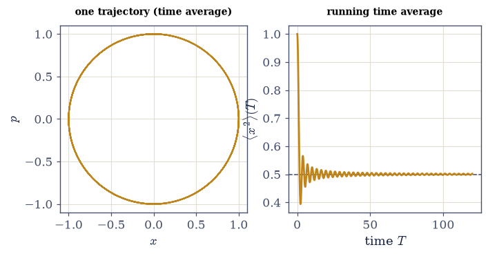
Fig. 422 The two averages. Left: along a single trajectory on the energy surface (the ellipse), the running time average \(\frac1T\int_0^T x^2\,dt\) accumulates moment by moment — what a measurement reports. Right: the ensemble average instead samples the whole surface at once (dots), following no trajectory. The ergodic hypothesis is the claim that the time average (the curve, settling to the dashed value) equals the ensemble average. The rest of the notebook tests it: exact for this oscillator, false for an integrable system, and restored by chaos.#
Exercise 2 — Liouville’s theorem: the measure the flow preserves (worked)#
Before comparing the two averages we must say which ensemble measure is the right one, and Liouville’s theorem from §2.3 answers it. Hamiltonian flow is incompressible: take a blob of initial conditions and let every point flow, and the blob shears, stretches, and curls, but its phase-space area never changes Eq. 406 (Fig. 423). The consequence is decisive: a measure that is uniform over the energy surface is stationary — evenly spread states stay evenly spread — so the uniform (microcanonical) measure is the one the dynamics preserves, the natural equilibrium ensemble. This is why §5.4 weighted every microstate equally. But notice what Liouville does not say: it constrains the whole blob, never a single point. One trajectory could still be trapped on part of the surface forever. That gap is exactly where ergodicity lives.
The test flow is the pendulum \(H=p^2/2-\cos q\), genuinely nonlinear, and the blob is a
ring of \(400\) points of radius \(0.28\) centred at \((q,p)=(0,1.65)\) — close to the separatrix,
where the period varies steeply with amplitude and the shear is violent. A ring that dense is
needed because the polygon edges must stay short while it stretches tenfold; the enclosed area
is then read by the Setup’s shoelace polygon_area.
Evolve every ring point under the pendulum flow with
scipy.integrate.solve_ivp, sampling the same \(60\) frame times over \(10\) time units so one integration serves both the area measurement and the animation.Measure the enclosed area at every frame and confirm the final area matches the initial one to
rtol=1e-3: the ring distorts dramatically and its area does not move — Liouville’s theorem, watched directly.
ring area at t=0:  0.246291
ring area at t=10: 0.246162
area ratio (final/initial) = 0.999477   (Liouville: exactly 1)
Validation 2#
✓ the phase-space area of a blob is conserved under Hamiltonian flow (Liouville) [got 0.246162 vs expected 0.246291 (rtol=0.001, atol=1e-09)]
True
Fig. 423 Liouville’s theorem, animated. A ring of \(400\) initial conditions (amber) is carried by the nonlinear pendulum flow; it shears and curls into a comma, yet the enclosed phase-space area (printed) holds fixed to three digits. Incompressibility is why a uniform spread over the energy surface stays uniform — the microcanonical measure of §5.4 is the one the dynamics preserves. What Liouville does not fix is whether any single point eventually visits the whole surface: that is ergodicity, taken up next.#
Exercise 3 — The oscillator is ergodic: time average = ensemble average (worked)#
Now the cleanest possible test of the ergodic equality. For one oscillator the energy surface \(H=E\) is a single closed curve in \((x,p)\), and the trajectory traces that entire curve, over and over — so a single trajectory manifestly visits the whole surface, and the system is ergodic trivially. We can therefore predict the time-average distribution of position analytically: the particle moves slowest near the turning points \(\pm A\), so it spends most of its time there, and the density is the arcsine law \(p(x)=1/\pi\sqrt{A^2-x^2}\) Eq. 407 (Fig. 424). This is also the microcanonical distribution — the fraction of the energy surface at each \(x\) — so the two agree by construction. Two independent readings confirm it: the empirical and analytic cumulative distributions coincide (comparing CDFs sidesteps the binning singularity at \(\pm A\)), and \(\langle x^2\rangle\) comes out the same as a time average and as the ensemble value \(E/m\omega^2\).
The trajectory is the same oscillator run out to \(T=200\pi\), about a hundred periods, sampled
at \(300\,000\) points and integrated a little tighter (rtol=1e-11, atol=1e-13) because a
distribution needs more of the trajectory than a mean does. Sorting \(n\) samples and pairing the
\(i\)-th with \((i-\tfrac12)/n\) is the empirical CDF; the arcsine CDF it is compared against is
\(F(x)=\tfrac12+\arcsin(x/A)/\pi\) Eq. 407, and the arcsine law’s own mean of \(x^2\) is
\(A^2/2\).
From that long trajectory build the empirical CDF of position (
numpy.sort), compare it with the arcsine CDF, and confirm the maximum difference over all samples is tiny.Check that the time-averaged \(\langle x^2\rangle\) equals the ensemble value \(A^2/2=E/m\omega^2\).
max |CDF_empirical − CDF_arcsine| = 5.00e-06   (time average matches microcanonical)
⟨x²⟩ time average  = 0.50000
⟨x²⟩ ensemble A²/2 = 0.50000   (= E/mω² = 0.50000)
Validation 3#
✓  the oscillator's time-average position law matches the microcanonical arcsine (via the CDF)   [got 4.99503e-06 vs expected 0 (rtol=1e-06, atol=0.01)]
✓  ⟨x²⟩ is the same as a time average and as an ensemble average   [got 0.500002 vs expected 0.5 (rtol=0.01, atol=1e-09)]
True
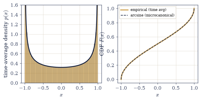
Fig. 424 The oscillator is ergodic, exactly. Left: the histogram of position along one long trajectory (amber) lands on the arcsine law \(p(x)=1/\pi\sqrt{A^2-x^2}\) (dark), which piles up at the turning points where the motion is slowest. Right: the empirical cumulative distribution and the microcanonical CDF \(F(x)=\tfrac12+\arcsin(x/A)/\pi\) are indistinguishable (max difference \(\sim10^{-6}\)). Because the trajectory is the whole energy curve, the time average and the ensemble average are the same — the bedrock case the harder ones are measured against.#
Exercise 4 — An integrable system is not ergodic: motion on a torus (worked)#
Here the ergodic equality fails, and seeing exactly why is the point. Take two uncoupled oscillators with an irrational frequency ratio. Because they never exchange energy, each oscillator’s energy \(E_x\) and \(E_y\) is conserved separately — that is a second invariant beyond the total energy Eq. 408. The total energy alone would allow the system to roam a three-dimensional surface, but the two separate conservation laws pin the motion to a two-dimensional torus: the trajectory winds densely around it (the Lissajous figure) yet never leaves it (Fig. 425). On the \((E_x,E_y)\) plane the motion sits at a single point for all time — it never explores any other division of the energy. So the time average of, say, \(x^2\) is fixed by which torus we started on; change the initial amplitudes and it changes. The time average depends on initial conditions, and there is no single ensemble value it equals. Integrable means non-ergodic.
The pair below has frequencies \(\omega_x=1\) and \(\omega_y=\sqrt2\): an irrational ratio, so the
trajectory never closes and covers its torus densely rather than retracing a loop. It starts at
amplitudes \((x,y)=(1,0.6)\) with both momenta zero, and runs for \(200\) time units at
rtol=1e-11, atol=1e-13. Each oscillator’s energy is \(E_i=\tfrac12(p_i^2+\omega_i^2q_i^2)\),
and the quantity that decides the question is the range of each over the whole run: a
conserved \(E_x\) and \(E_y\) is a second invariant, and a second invariant is the torus.
Integrate the two-oscillator system and form \(E_x\) and \(E_y\) along the trajectory.
Confirm each is separately conserved — their ranges over the whole run are \(\sim10^{-11}\) — and that the motion is a bounded torus which never fills the energy surface.
E_x = 0.5000 (range 3.63e-12),  E_y = 0.3600 (range 5.12e-11)
each oscillator's energy is separately conserved — the motion is locked to one torus
→ the time average depends on which torus (initial conditions): the system is NOT ergodic
Validation 4#
✓ each oscillator's energy is separately conserved — a second invariant confines the motion to a torus (non-ergodic) [max|Δ| = 5.11638e-11 (rtol=1e-06, atol=1e-06)]
True
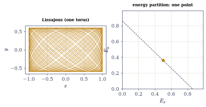
Fig. 425 An integrable system stays on a torus. Left: the trajectory in the \((x,y)\) plane is a Lissajous figure that winds densely through a bounded box but never escapes it. Right: on the \((E_x,E_y)\) plane the motion is a single fixed point (amber) — the two energies are separately conserved, so the system never explores any other partition of the total energy (the dashed line \(E_x+E_y=E\)). The time average is set by this one point; start on a different torus and it differs. Non-ergodic, exactly because there is a second invariant.#
Exercise 5 — The Hénon–Heiles system: regular and chaotic regimes (worked)#
To find genuine ergodicity we need a system that is not integrable, and the Hénon–Heiles model is the classic. It describes a star moving in the plane of a galaxy, \(H=\tfrac12(p_x^2+p_y^2)+\tfrac12(x^2+y^2)+x^2y-\tfrac13 y^3\) — two oscillators coupled by the cubic terms — and its potential is a triangular well that confines bound motion for energies below the escape value \(E=1/6\) (Fig. 426). The coupling destroys the second invariant: there is no \(E_x\), no \(E_y\), only the total energy. At low energy the system stays nearly regular (the tori survive, deformed); near the escape energy it becomes chaotic. Before we can study either regime we need an integrator we trust, so the first check is that energy is conserved — for a 2-degree-of-freedom nonlinear system, holding \(H\) fixed to \(\sim10^{-10}\) over hundreds of time units is the certificate that the dynamics, not numerical drift, is what we are seeing.
The two working energies are \(E=0.04\) (low, regular) and \(E=0.16\) (just under the escape value
\(1/6\approx0.167\), chaotic), and every run in this notebook starts on the section plane \(x=0\):
the Setup’s henon_heiles_ic chooses \(p_x\ge0\) from \(H=E\) so the initial point sits exactly on
the requested energy surface. Both runs cover \(500\) time units, sampled at \(5000\) points.
Integrate Hénon–Heiles at both energies with
scipy.integrate.solve_ivp(DOP853).Evaluate
henon_heiles_energyalong each trajectory and confirm the largest \(|H-E|\) stays at the \(\sim10^{-10}\) level, so everything that follows is dynamics rather than drift.
E = 0.04: max |H − E| over the trajectory = 5.47e-11
E = 0.16:  max |H − E| over the trajectory = 3.07e-10
energy held to ~1e-10 — the integrator is faithful; what we see is dynamics, not drift
Validation 5#
✓ the high-accuracy integration conserves the Hénon–Heiles energy [got 3.06984e-10 vs expected 0 (rtol=1e-06, atol=0.001)]
True
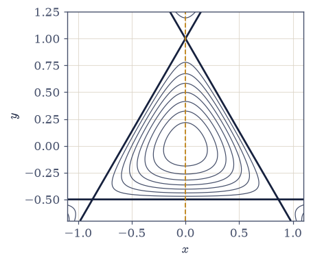
Fig. 426 The Hénon–Heiles setup. Contours of the potential \(V=\tfrac12(x^2+y^2)+x^2y-\tfrac13y^3\): a harmonic bowl near the origin that opens into a triangular well with three escape channels at the energy \(E=1/6\) (heavy contour). Bound motion lives inside, on the energy surface \(H=E\). The dashed line is the Poincaré-section plane \(x=0\) used in the next exercise to read off the geometry of the motion. The cubic coupling removes the separate \(E_x,E_y\) invariants of the uncoupled case — opening the door to chaos.#
Exercise 6 — Poincaré sections: tori versus the chaotic sea (worked)#
The Poincaré section turns a tangled four-dimensional flow into a picture you can read at a glance, and it is the iconic image of the integrable-to-chaotic transition. Each time a trajectory pierces the plane \(x=0\) moving in the \(+x\) direction, we drop a dot at its \((y,p_y)\) Eq. 408,Eq. 409. A trajectory on a surviving torus pierces the plane on a smooth closed loop — its dots trace a curve. A chaotic trajectory has no such invariant surface to live on, so its dots scatter and fill an area (Fig. 427). At low energy (\(E=0.04\)) every trajectory gives nested closed curves: the motion is regular. Near the escape energy (\(E=0.16\)) a single trajectory’s points spray across a two-dimensional sea: the motion is chaotic, and that one trajectory is already exploring most of the accessible surface — the geometric signature of (approximate) ergodicity.
A section is found by event detection rather than by searching the sampled output: give
scipy.integrate.solve_ivp an event function that returns \(x\), and it locates every zero of
that function to integrator accuracy and reports the full state there in sol.y_events.
Setting event.direction = 1.0 keeps only the crossings with \(x\) increasing, which is the
\(p_x>0\) half of the section, and capping max_step keeps the solver from striding over a
crossing between two internal steps. The state ordering is \((x,p_x,y,p_y)\), so the section
coordinates are its last two components.
Write
poincare_section(rhs, s0, t_max, max_step=0.5): integrate the flow froms0and return the arrays \((y,p_y)\) of every crossing of the plane \(x=0\) with \(p_x>0\), and an empty pair if the trajectory never crosses.Pool the sections of five initial conditions at \(E=0.04\) and five at \(E=0.16\) (\(t_{\max}= 2500\) each), and quantify the contrast with a grid-occupancy measure (
numpy.histogram2d, \(40\times40\) cells): the chaotic section fills several times more cells than the regular one.
low energy  E=0.04: 1953 points, grid occupancy = 0.111  (thin curves: tori)
high energy E=0.16: 1765 points, grid occupancy = 0.429  (filled sea: chaos)
the chaotic section fills 3.9× more of the plane
Validation 6#
✓ the Poincaré section is thin curves (tori) at low energy and a space-filling sea (chaos) at high energy
True
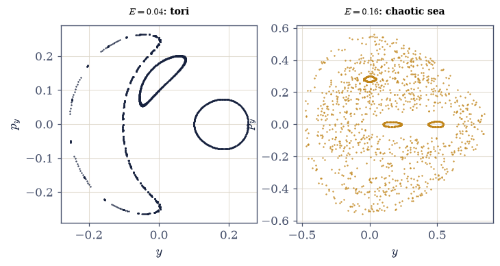
Fig. 427 The integrable-to-chaotic transition, on the Poincaré plane \(x=0\). Left (\(E=0.04\)): every trajectory pierces the plane on a nested closed curve — surviving tori, regular motion, each initial condition trapped on its own invariant loop. Right (\(E=0.16\)): a few trajectories’ crossings scatter across a two-dimensional sea, filling several times more of the plane. A single chaotic trajectory already wanders over most of the accessible surface — this is what (approximate) ergodicity looks like, and the engine behind it is measured next.#
Exercise 7 — The Lyapunov exponent: measuring chaos (worked)#
What makes a single chaotic trajectory fill the surface? Sensitive dependence on initial conditions: two trajectories that start a hair apart separate exponentially, \(\lvert\delta(t) \rvert\sim\lvert\delta_0\rvert\,e^{\lambda t}\), and the rate \(\lambda\) is the largest Lyapunov exponent Eq. 409. A positive \(\lambda\) is the quantitative fingerprint of chaos — and it is precisely the mechanism of effective ergodicity, because exponential stretching is what folds one trajectory through every corner of the accessible surface. We measure \(\lambda\) by Benettin’s trick: run a reference trajectory and a shadow a tiny distance away, and every short interval record how much their separation grew and then rescale the shadow back, so it tracks the local stretching forever without saturating (Fig. 428). At high energy \(\lambda\) is clearly positive; at low energy it decays toward zero (regular motion separates only as a power of \(t\), so the running estimate drifts down as \(\sim\ln t/t\)).
That renormalization loop was built from scratch in §2.11,
where it was checked against Lorenz’s tabulated \(\lambda_1=0.9056\); here it is a meter rather
than a lesson, and the Setup’s lyapunov_exponent is that same construction. It is applied for
\(t_{\rm total}=3000\) time units, long enough that the average has converged: the fine detail of
a chaotic trajectory differs between machines — that is sensitive dependence doing its job — but
the averaged exponent does not.
Estimate \(\lambda\) at \(E=0.16\) and at \(E=0.04\), both from initial conditions on the section plane.
Confirm it is clearly positive in the chaotic regime and near zero in the regular one, the stretching that folds one trajectory through the whole surface.
λ at E=0.16 (chaotic) = 0.1046   (clearly positive)
λ at E=0.04 (regular) = 0.0016   (near zero)
ratio = 65× — exponential stretching is the engine of effective ergodicity
Validation 7#
✓ the Lyapunov exponent is positive in the chaotic regime and near zero in the regular regime
True
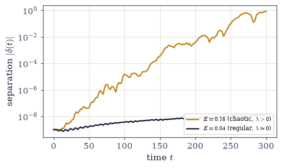
Fig. 428 Measuring chaos. The separation between two initially-adjacent trajectories, tracked by Benettin’s renormalization, against time. At \(E=0.16\) (amber) it grows exponentially — a straight line on this log axis, slope \(\lambda\approx0.10\) — the signature of chaos and sensitive dependence on initial conditions. At \(E=0.04\) (dark) it barely grows, \(\lambda\approx0\), the hallmark of regular motion. The positive exponent is exactly what folds one trajectory through the whole energy surface, turning a single orbit into an explorer of phase space — the mechanism that makes a chaotic system effectively ergodic.#
Exercise 8 — Time average meets ensemble average in the chaotic regime (student)#
Now we close the loop the whole notebook has been building toward. In the chaotic regime a single trajectory explores (most of) the energy surface, so its time average of an observable should converge to the ensemble average over that surface Eq. 405,Eq. 409 — the ergodic equality, restored by chaos. We test it on \(\langle y^2\rangle\) at \(E=0.16\). The ensemble average is computed directly from the microcanonical measure: by Liouville the measure is uniform in the accessible configuration region (with the momentum direction uniform), so \(\langle y^2 \rangle_{\rm ens}\) is just the area-weighted average of \(y^2\) over \(\{V(x,y)\le E\}\). The time average comes from long chaotic trajectories. They agree to a few percent (Fig. 429) — and crucially, different chaotic starting points give the same time average, the true mark of ergodicity. Contrast the integrable two-oscillator system, whose time average is set by the initial torus and refuses to settle on any common value. Realistic matter is chaotic; that is why the ensemble averages of §5.4 predict what is measured.
The ensemble side is a Monte Carlo area average: draw points uniformly from a box containing the well (\(x\in[-0.8,0.8]\), \(y\in[-0.6,1.1]\)), keep those with \(V(x,y)\le E\) — the region the motion can reach — and average \(y^2\) over the survivors. Two million points make the estimate steady to the percent the comparison needs. The time side is five trajectories of \(5000\) time units from different points of the chaotic sea, and the integrable comparison run is the uncoupled pair again, started at two different amplitudes.
Estimate \(\langle y^2\rangle_{\rm ens}\) by that sampling (
numpy.random.default_rng, seeded so the number is reproducible).Average \(y^2\) over the five long chaotic trajectories, and confirm the two numbers agree to within about ten percent — and that the five per-trajectory values agree with each other, which is the part that says ergodic rather than merely close.
Show the integrable system’s time average of \(x^2\) is instead initial-condition-dependent: the same measurement at two amplitudes gives two different answers.
⟨y²⟩ ensemble (phase-space average) = 0.1126
⟨y²⟩ time average over 5 chaotic trajectories = 0.1194
  per-trajectory: [0.1097, 0.1696, 0.1107, 0.1215, 0.0853] — different starts, same average (ergodic)
  agreement: 6.0%
integrable ⟨x²⟩ time average: A=1.0 → 0.501, A=0.5 → 0.125 (IC-dependent: NOT ergodic)
Validation 8#
✓ in the chaotic regime the time average converges to the ensemble average — ergodicity, restored by chaos [got 0.119367 vs expected 0.112604 (rtol=0.1, atol=1e-09)]
True
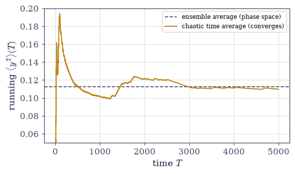
Fig. 429 Ergodicity, restored by chaos. The running time average \(\langle y^2\rangle(T)\) along a chaotic Hénon–Heiles trajectory at \(E=0.16\) (amber) wanders but converges toward the microcanonical ensemble average (dashed), computed independently by sampling the energy surface — they agree to a few percent, and different chaotic starts give the same limit. For comparison, the integrable two-oscillator time average of \(x^2\) (dark, two different initial amplitudes) settles to different values, each fixed by its torus. Chaos makes one trajectory stand in for the whole ensemble; integrability does not. This is the licence under statistical mechanics.#
Exercise 9 — Why the ensembles are allowed (synthesis)#
Stand back and see what we have established. Statistical mechanics computes ensemble averages — integrals over the energy surface — but every measurement is a time average along one trajectory. The bridge between them is ergodicity, and we have tested it from every side. Liouville’s theorem (§2.3) told us which measure the dynamics preserves, singling out the uniform microcanonical measure of §5.4 as the equilibrium one. The harmonic oscillator showed the time and ensemble averages can be exactly equal — its trajectory is the whole energy curve. Two uncoupled oscillators showed the equality can fail — a second invariant traps the motion on a torus, and the time average remembers its initial conditions. The Hénon–Heiles system showed what rescues it — chaos, a positive Lyapunov exponent, a single trajectory spilling across the whole surface so the time average returns to the ensemble value. Realistic many-body systems are overwhelmingly chaotic, hence effectively ergodic, and that — not a theorem — is why the microcanonical ensemble describes real matter. The ensembles to come rest on the same foundation.
There is no new computation here: the argument is the result. We compute over all of phase space and trust that one trajectory, given time, visits it all. For a chaotic system it does — we measured it — and that trust is the foundation under everything that follows. Where it breaks, so does the ensemble description, which is the warning the Ising capstone will take up as ergodicity breaking.
Notebook summary#
Statistical mechanics computes phase-space averages but predicts time averages; this notebook examined the assumption — ergodicity — that lets it, building each step on Volume II’s Hamiltonian dynamics and Liouville’s theorem.
Two kinds of average Eq. 405: the time average \(\bar A\) along a trajectory (what is measured) versus the ensemble average \(\langle A\rangle\) over the energy surface (what is computed); the ergodic hypothesis is \(\bar A=\langle A\rangle\).
Liouville’s theorem Eq. 406: Hamiltonian flow is incompressible (a pendulum blob conserves its area to three digits), so the uniform measure on the energy surface is stationary — the equilibrium measure of §5.4. But it does not by itself guarantee ergodicity.
The oscillator Eq. 407: trivially ergodic; the time-average position is the arcsine law, matching the microcanonical CDF to \(\sim10^{-6}\), and \(\langle x^2\rangle=E/m\omega^2\) both ways.
Integrable = non-ergodic Eq. 408: two uncoupled oscillators conserve \(E_x,E_y\) separately (ranges \(\sim10^{-11}\)), confining the motion to a torus; the time average depends on initial conditions.
Chaos restores ergodicity Eq. 409: Hénon–Heiles is regular at \(E=0.04\) and chaotic at \(E=0.16\) (energy conserved to \(\sim10^{-10}\)); its Poincaré section turns from nested curves into a space-filling sea, its Lyapunov exponent from \(\approx0\) to \(\approx0.10\), and the chaotic time average of \(\langle y^2\rangle\) converges to the ensemble average (a few percent).
The ensemble method is licensed because realistic systems are chaotic enough to be effectively ergodic — an assumption, demonstrable and breakable, not a theorem.
Outlook#
Mixing and the approach to equilibrium. A stronger property than ergodicity — not just that a trajectory visits everywhere, but that any initial distribution relaxes to uniform — and the timescales on which a system forgets where it started.
Molecular dynamics. The practical face of the time average: a single long trajectory, integrated exactly as we did here, standing in for the ensemble — the bridge to the simulation methods of this volume and to materials modelling.
The other derivatives of entropy (§5.6). With the ensemble method justified, pressure and chemical potential as \(\partial S/\partial V\) and \(\partial S/\partial N\), and the fundamental thermodynamic relation — the rest of thermodynamics from the same \(S=k\ln\Omega\).
The canonical ensemble. Summing the Boltzmann factor of §5.4 over a system’s states into the partition function \(Z\), from which \(\ln Z\) generates all thermodynamics — developed later in the volume, and resting on the same ergodic foundation examined here.
Ergodicity breaking (the Ising capstone, §5.10). When a system gets trapped in part of phase space — a glass, or a ferromagnet frozen in one magnetization sector below \(T_c\) — the time and ensemble averages part ways, and the ensemble description must be handled with care.
Cross-reference §2.3 (Hamiltonian flow and Liouville’s theorem) and §5.4 (the microcanonical ensemble).