2.5 Scattering and the Rutherford Cross-Section

Elementary Computational Physics

Volume II — Analytical Mechanics Notebook 2.5

Unbound orbits and how a beam scatters: impact parameter, deflection angle, and the differential cross-section — recovering Rutherford's famous 1/sin⁴(θ/2) law from classical mechanics.

Level · intermediate   •   Est. · 75–100 min

Raymond Amador v1.4.0  ·  2026-07-31  ·  CC BY 4.0 (text) / MIT (code)

Notebook overview

§2.4 read the effective potential as a 1-D energy diagram and classified orbits by energy: \(E<0\) gave the bound ellipses, and \(E\ge0\) was set aside as the scattering states. This notebook is that \(E>0\) sequel. A particle now comes in from far away, swings once past the force centre on an unbound hyperbola, and leaves: deflected through a scattering angle \(\theta\) that depends on how closely it was aimed, the impact parameter \(b\).

The payoff is one of the most consequential formulas in physics. A beam of particles carries a spread of impact parameters; geometry maps that spread of \(b\) onto a spread of outgoing angles \(\theta\), and the differential cross-section \(d\sigma/d\Omega\) records how many particles emerge per unit solid angle. For the Coulomb potential this is the Rutherford formula \(d\sigma/d\Omega\propto 1/\sin^4(\theta/2)\): the long tail of large-angle events that, measured in Geiger and Marsden’s gold-foil experiment, revealed the atomic nucleus. We derive it from the same central-force machinery as §2.4, with no quantum mechanics anywhere.

We reuse the 2-D integrator from §1.4/§2.4; you write the deflection(b, E) that fires one particle from far away and reports how much it turned (Exercise 1), and the rest of the notebook puts it to work: a single hyperbolic trajectory, the deflection law \(\tan(\theta/2)=k/(2Eb)\), the Rutherford cross-section as the centrepiece, an animated beam fanning out by angle, an attractive-vs-repulsive comparison, and the divergent total cross-section that announces the infinite range of the Coulomb force.

A deliberate numerical lesson. Rutherford’s formulas assume the particle starts at infinity. We must launch from a finite distance, where the particle already feels the \(1/r\) tail, so trajectory-measured angles come out systematically a little low, and the more so for large \(b\) (those orbits skim the tail for longer). The trajectory checks below therefore run at \(\sim2\%\) tolerance, while the purely analytic cross-section check (Exercise 4) is exact to \(\sim10^{-8}\) because it never integrates a trajectory at all. Watching where the error does and does not appear is half the point of the notebook.

How to read the checks. Each exercise ends with a validation that compares a computed result to an expected physical fact. A ✗ does not by itself mean the physics is wrong: it means the output didn’t match what the check expected, which may be a real error, a different-but-valid convention (a sign, a unit, an array order), or simply too tight a tolerance. Treat a ✗ as a prompt to locate the discrepancy; passing is strong evidence of correctness, not proof.

Scope. This is a working review, not a textbook chapter. For the full theory of central-force scattering and the cross-section, see Nolting, Theoretical Physics 2 [Nol16], Goldstein, Poole & Safko [GPS02] (ch. 3), and Landau & Lifshitz, Mechanics [LL76] (§18–19).

Theory in brief

The scattering setup

A beam of particles, each of energy \(E>0\), comes in from infinity travelling parallel to a chosen axis. A given particle is offset from the axis through the centre by the impact parameter \(b\): the perpendicular distance at which it would pass the centre if there were no force. The central force bends its path into an unbound hyperbola, and it departs to infinity having turned through the scattering angle \(\theta\) (see Fig. 138). The whole problem is to find the map \(b\mapsto\theta\), and then what it does to a beam.

Because the orbit is unbound, the conserved angular momentum is fixed by the incoming conditions: \(L=\mu v_\infty b\) with \(v_\infty=\sqrt{2E/\mu}\).

The deflection angle

Integrating the radial motion Eq. 149 from the distance of closest approach \(r_{\min}\) (the single turning point) out to infinity, and doubling by symmetry, gives the deflection-angle integral

(154)\[\theta(b) = \pi - 2\!\int_{r_{\min}}^{\infty} \frac{L/r^2}{\sqrt{\,2\mu\bigl(E-V_{\mathrm{eff}}(r)\bigr)}}\;dr , \qquad V_{\mathrm{eff}}(r)=V(r)+\frac{L^2}{2\mu r^2}.\]

For the repulsive Coulomb potential \(V(r)=k/r\) (with \(k>0\)) this integral has a closed form (Landau & Lifshitz, Mechanics [LL76], §19, carries the integration out): the orbit is a hyperbola whose asymptotes make the simple relation

(155)\[\tan\!\frac{\theta}{2} = \frac{k}{2Eb} ,\]

so \(b\to0\) (a head-on aim) gives \(\theta\to\pi\) (back-scatter), and \(b\to\infty\) gives \(\theta\to0\) (no deflection). Inverting, \(b(\theta)=\dfrac{k}{2E}\cot\dfrac{\theta}{2}\).

The differential cross-section

Particles entering through the annulus between \(b\) and \(b+db\) (area \(2\pi b\,|db|\)) all emerge between \(\theta\) and \(\theta+d\theta\) (solid angle \(d\Omega=2\pi\sin\theta\,|d\theta|\)). Equating the counts defines the differential cross-section

(156)\[\frac{d\sigma}{d\Omega} = \left|\frac{b}{\sin\theta}\,\frac{db}{d\theta}\right| .\]

Substituting \(b(\theta)\) from Eq. 155 and its derivative \(db/d\theta=-(k/4E)\csc^2(\theta/2)\) collapses everything to the Rutherford formula

(157)\[\frac{d\sigma}{d\Omega} = \left(\frac{k}{4E}\right)^{2}\frac{1}{\sin^{4}(\theta/2)} .\]

What the cross-section means, and its catastrophe

\(d\sigma/d\Omega\) has units of area per steradian: it converts the incident beam flux into the rate of particles scattered into a detector at angle \(\theta\). The \(1/\sin^4(\theta/2)\) divergence as \(\theta\to0\) is the historic signature: a sharp forward pile-up with a long tail of large-angle events that only a small, hard, charged core could produce. Integrating it over all angles, the total cross-section diverges, because the Coulomb force has infinite range: every particle, however large its \(b\), is deflected a little. A physical target screens the charge at large \(r\) and restores a finite total: the link to the screened (Yukawa) potential and, ultimately, the quantum Born approximation of Volume VI.

---

Setup

We work in reduced units \(\mu=1\) and a repulsive Coulomb strength \(k=1\), so \(V(r)=k/r\) and the deflection law Eq. 155 is just \(\tan(\theta/2)=1/(2Eb)\). Setup holds that units choice, the potential itself, the 2-D Newtonian state derivative restated from §1.4 with the Coulomb sign (\(\mathbf a = k\,\mathbf r/r^3\): outward for \(k>0\), inward for \(k<0\)), and the closed-form deflection law the measurements are checked against. The notebook’s own machinery is not here: you write deflection, which fires one particle from far away and reports how much it turned, in Exercise 1, and the cross-section itself is assembled in Exercise 4.

The Setup below holds this notebook’s data and instruments — nothing you are asked to build. It is collapsed so the building stays yours; expand it whenever you want the details.

Show code cell source

Hide code cell source

import numpy as np
from scipy.integrate import solve_ivp
import matplotlib.pyplot as plt
from matplotlib.animation import FuncAnimation

from ecp import draw, validate
from ecp.animate import show

MU = 1.0  # data: reduced units, μ = 1
K = 1.0  # data: repulsive Coulomb strength k (V = k/r)


# instrument: the model's given potential, quoted from the theory above — it only
# turns a radius into a potential energy so the conserved-energy series can be
# formed, and is nobody's lesson here.
def V(r, k=K):
    """Coulomb potential energy V(r) = k/r (repulsive for k > 0).

    Parameters
    ----------
    r : float or numpy.ndarray
        Separation.
    k : float, optional
        Coupling strength.

    Returns
    -------
    float or numpy.ndarray
        The potential energy.
    """
    return k / r


# built from scratch in §1.4 (Exercise 1's `rhs`, the same 2-D Newtonian state
# derivative with the gravitational sign) and restated in §2.4; restated here as an
# instrument, with the Coulomb acceleration and k carried as an argument. The
# `deflection` you write in Exercise 1 is what drives it.
def cartesian_rhs(_t, s, k):
    """2-D Coulomb state derivative; acceleration a = k·r/r^3 (μ = 1)."""
    x, y, vx, vy = s
    r3 = (x * x + y * y) ** 1.5
    return [vx, vy, k * x / r3, k * y / r3]


# instrument: the closed form quoted in the theory above
# ({eq}`eq-rutherford-angle`, integrated in Landau & Lifshitz §19) — the reference
# the trajectory measurements are checked against, not machinery any exercise builds.
def theta_analytic(b, E, k=K):
    """Closed-form Rutherford deflection angle, tan(θ/2) = |k|/(2·E·b) (eq-rutherford-angle).

    Parameters
    ----------
    b : float or numpy.ndarray
        Impact parameter.
    E : float
        Energy.
    k : float, optional
        Coupling.

    Returns
    -------
    float or numpy.ndarray
        The deflection angle.
    """
    return 2.0 * np.arctan(abs(k) / (2.0 * E * b))

Exercise 1 — The scattering geometry

Before any numbers, fix the picture. A particle of energy \(E>0\) approaches along a line offset from the centre by the impact parameter \(b\); it is repelled, swings around the centre once, and leaves along an outgoing asymptote tilted by the scattering angle \(\theta\) from its original direction. The closer the aim (smaller \(b\)), the harder the kick and the larger \(\theta\). The deflection integral Eq. 154 turns this geometry into the function \(\theta(b)\) we spend the rest of the notebook exploring.

Measuring \(\theta\) from a trajectory forces one decision the theory never has to make: where to start. The formulas assume a launch at infinity; we must launch from far out on the \(-x\) axis at a finite \(x_0=-\max(200,\,100\,|b|)\) — far, and farther still for large \(b\), precisely to keep the finite-distance systematic flagged above down at the percent level. The natural stopping point is symmetric with the start: the encounter is over once the particle has climbed back out to its launch radius \(r_0\), which scipy.integrate.solve_ivp will detect for us as a terminal event on the outgoing crossing (returned.terminal = True, returned.direction = 1.0), and the outgoing direction is then read straight off the final velocity. A scattering state must do two things a bound orbit never does: keep \(E>0\), and leave — return to a large radius instead of staying trapped.

1. Write deflection(b, E, k=K, x0=None, n_eval=2000): launch at impact parameter \(b\) with the asymptotic speed \(v_\infty=\sqrt{2E/\mu}\), integrate cartesian_rhs with DOP853 at tight tolerances until the terminal event fires, and return the deflection angle \(\theta=\mathrm{atan2}(v_y,v_x)\) measured from the incoming \(+x\) direction, together with the sampled times, the path \((x,y)\), and the energy series \(\tfrac12 v^2+V(r)\) along it (ask for dense_output and you can resample the whole path on a uniform grid once the event has stopped it). Write this one yourself — the implementation is the lesson.

2. Integrate one scattering trajectory with it and confirm it is an unbound state: it comes in from large \(r\) and returns to large \(r\) (it does not stay trapped), with \(E>0\).

3. Study the geometry (incoming and outgoing asymptotes, impact parameter \(b\), scattering angle \(\theta\)) drawn in Fig. 138.

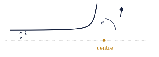
Fig. 138 Central-force scattering geometry: a particle of energy \(E>0\) comes in from the left (dashed incoming asymptote) at impact parameter \(b\) — the perpendicular offset from the line through the scattering centre (amber). It is repelled, rounds the centre at the distance of closest approach, and leaves along the outgoing asymptote (dashed), deflected through the scattering angle \(\theta\) from its original direction. Smaller \(b\) means a closer approach and a larger \(\theta\).

Validation 1 — the trajectory is an unbound scattering state

A scattering state must do two things a bound orbit never does: have \(E>0\), and leave: return to a large radius rather than stay trapped. We confirm the integrated trajectory reaches back out beyond a threshold radius.

final radius r = 200.00  (threshold 50.0),  E = 1.0050
✓  the trajectory is an unbound scattering state (E>0, returns to large r)   [r_final = 200.0, E = 1.0050]

True

Exercise 2 — A single scattering trajectory (worked)

Here is the scattering event in full: one particle, one impact parameter, the hyperbolic path past the centre. The two asymptotes (the straight lines the particle follows long before and long after the encounter) meet at the scattering angle \(\theta\). Along the way, the energy \(E=\tfrac12\mu v^2+k/r\) must stay exactly constant: the force does no net work over the round trip, it only redirects the momentum. We integrate with the deflection you wrote in Exercise 1, draw the path with its asymptotes and \(\theta\) marked, and verify energy conservation along the orbit (Fig. 139).

This is a worked exercise; you build the beam animation in Exercise 5.

scattering angle: numeric θ = 53.015°,  analytic = 53.130°
energy drift: 9.26e-12  (about E≈1.005)

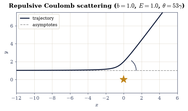
Fig. 139 A single repulsive-Coulomb scattering trajectory (\(b=1\), \(E=1\), \(k=1\)): the particle (blue) comes in along the lower dashed incoming asymptote, rounds the centre (amber) at its distance of closest approach, and departs along the upper dashed outgoing asymptote, deflected through the scattering angle \(\theta\). The hyperbola is symmetric about the line to closest approach, and the energy is conserved to the integrator tolerance along the whole path.

Validation 2 — energy is conserved along the trajectory

Scattering conserves energy exactly: the Coulomb force is conservative, so \(E=\tfrac12\mu v^2+k/r\) may drift only at the integrator’s tolerance over the whole encounter.

✓  energy conserved along the scattering trajectory   [max relative drift = 5.58602e-12 (limit 1e-06)]

True

Exercise 3 — Deflection angle vs. impact parameter

Now the central map \(b\mapsto\theta\). We fire a sweep of impact parameters at fixed energy, measure each outgoing angle from the trajectory, and test the closed-form law Eq. 155, \(\tan(\theta/2)=k/(2Eb)\). The agreement is the numerical proof that the Coulomb orbit really is the hyperbola the analysis claims.

This is also where the finite-distance systematic shows its face. Because we launch from a large but finite \(x_0\), every particle already feels the \(1/r\) tail at the start, so the measured deflection comes out a touch low, and the effect grows with \(b\) (those wide trajectories graze the tail for longer). We therefore validate at \(2\%\), and the residual creeps up with \(b\) in the data: the discrepancy is physics-of-the-method, not a coding bug. Contrast this with Exercise 4, whose check never integrates a trajectory and so is exact.

1. At \(E=1\), sweep \(b\) (numpy.linspace) and measure \(\theta(b)\) with the deflection you wrote in Exercise 1.

2. Overlay the numeric points on the analytic curve \(\theta=2\arctan(k/2Eb)\) (Fig. 140) and check they agree to \(2\%\).

  b      θ_num(°)   θ_law(°)   rel.err
 0.20   136.298   136.397     0.07%
 0.36   107.809   107.945     0.13%
 0.53    86.815    86.958     0.16%
 0.69    71.649    71.785     0.19%
 0.85    60.539    60.664     0.21%
 1.02    52.195    52.309     0.22%
 1.18    45.761    45.864     0.23%
 1.35    40.678    40.772     0.23%
 1.51    36.576    36.663     0.24%
 1.67    33.205    33.284     0.24%
 1.84    30.389    30.462     0.24%
 2.00    28.004    28.072     0.24%
max relative error over the sweep: 0.24%

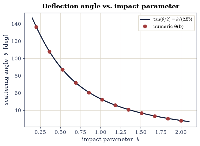
Fig. 140 Deflection angle vs. impact parameter for repulsive Coulomb scattering (\(E=1\), \(k=1\)): numerically measured angles \(\theta(b)\) (markers) lie on the closed-form law \(\tan(\theta/2)=k/(2Eb)\) (curve, Eq. 155). Small \(b\) (close aim) gives back-scatter \(\theta\to180°\); large \(b\) gives little deflection. The faint residual at large \(b\) is the finite-launch-distance systematic discussed in the text, not a numerical error in the law.

Validation 3 — the deflection follows \(\tan(\theta/2)=k/(2Eb)\)

The measured angles must match the closed-form law Eq. 155. The \(2\%\) tolerance is set deliberately to cover the finite-launch-distance systematic explained above: the method’s error, not the law’s.

✓  deflection angle follows tan(θ/2)=k/(2Eb)   [max|Δ| = 0.00249666 (rtol=0.02, atol=1e-09)]

True

Exercise 4 — The differential cross-section → Rutherford (worked, centrepiece)

This is the heart of the notebook. The deflection law \(b(\theta)\) is all we need: feeding it into Eq. 156, \(d\sigma/d\Omega=|(b/\sin\theta)(db/d\theta)|\), turns the single-particle geometry into the beam observable, and the algebra collapses to the Rutherford formula Eq. 157, \(d\sigma/d\Omega=(k/4E)^2/\sin^4(\theta/2)\).

Crucially, this exercise never integrates a trajectory. We use the analytic \(b(\theta)=(k/2E)\cot(\theta/2)\) and its closed-form derivative \(db/d\theta=-(k/4E)\csc^2(\theta/2)\), assemble \(d\sigma/d\Omega\) from Eq. 156, and compare to the closed form. So there is no finite-distance tail and no integrator drift: the check passes to machine precision, a sharp contrast with Exercise 3’s \(2\%\). That contrast is the lesson: numerical error enters only where one actually integrates dynamics.

1. From \(b(\theta)\) and its closed-form derivative, form \(d\sigma/d\Omega\) via Eq. 156 and compare to the Rutherford formula Eq. 157.

2. Plot \(d\sigma/d\Omega\) vs. \(\theta\) on a log axis (semilogy), showing the small-angle divergence (Fig. 141).

max relative error vs Rutherford formula: 5.92e-16

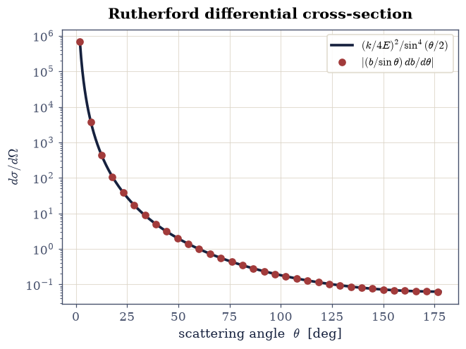
Fig. 141 The Rutherford differential cross-section (\(E=1\), \(k=1\)): \(d\sigma/d\Omega\) assembled from the geometric definition Eq. 156 using the analytic \(b(\theta)\) (markers) coincides with the closed form \((k/4E)^2/\sin^4(\theta/2)\) (Eq. 157, curve) over many decades. The steep rise toward small \(\theta\) is the \(1/\sin^4(\theta/2)\) forward divergence — the signature of a long-range \(1/r\) force, and the origin of the divergent total cross-section in Exercise 7.

Validation 4 — the cross-section is the Rutherford \(1/\sin^4(\theta/2)\) law

The geometric cross-section Eq. 156 built from \(b(\theta)\) must equal the closed-form Rutherford result Eq. 157 essentially exactly: this is a pure analytic identity, with no trajectory integrated, hence the \(10^{-4}\) tolerance (achieved to machine precision, \(\sim10^{-15}\)). Contrast Exercise 3’s \(2\%\).

✓  differential cross-section is the Rutherford 1/sin⁴(θ/2) law   [max|Δ| = 5.82077e-11 (rtol=0.0001, atol=1e-09)]

True

Exercise 5 — The beam picture (worked animation)

A cross-section is a statement about a beam, so let us fire one. Many particles start in a vertical line (a parallel beam) at a range of impact parameters and a common energy, and stream toward the centre. Watching them, the geometry of scattering becomes obvious: the inner particles (small \(b\)) get the hardest kick and fan out to large angles, while the outer ones sail past nearly undeflected. That monotonic ordering, small \(b\to\) large \(\theta\), is exactly what concentrates scattered particles in the forward direction and drives the Rutherford pile-up.

This is the worked animation; you build the attractive-vs-repulsive one in Exercise 6.

θ range across the beam: 18.7° (b=3.00) … 117.4° (b=0.30)

Once Loop Reflect

Fig. 142 Animation of a parallel beam scattering off a repulsive Coulomb centre (amber star; common energy \(E=1\), \(k=1\)): particles enter from the left at a range of impact parameters and fan out by angle. Small-\(b\) particles (nearest the axis) deflect most strongly, large-\(b\) particles barely turn — the monotonic ordering \(b\downarrow\Rightarrow\theta\uparrow\) that underlies the forward-peaked Rutherford cross-section.

Validation 5 — energy conserved across the beam, and \(b\downarrow\Rightarrow\theta\uparrow\)

Two physical facts about the animated beam data (not the animation object): every particle conserves its energy, and the deflection is monotonic: sorting by impact parameter, the scattering angle decreases as \(b\) grows. The monotonicity is the mechanism behind the forward-peaked cross-section.

✓  every beam particle conserves energy   [max|Δ| = 2.2442e-12 (rtol=0.0001, atol=1e-09)]
✓  smaller impact parameter gives larger deflection (monotonic θ(b))   [θ decreases from 117.4° to 18.7° as b grows]

True

Exercise 6 — Attractive vs. repulsive (student-implemented animation)

A remarkable fact hides in the Rutherford formula: it depends on \(k\) only through \(k^2\), so an attractive Coulomb force (\(k<0\), e.g. an electron on a nucleus) produces the same cross-section as the repulsive one. The deflection magnitude obeys the same \(|\tan(\theta/2)|=|k|/(2Eb)\), only the sense of the bend differs: the repelled particle veers away from the centre, the attracted one swings toward it and whips around the far side. The cross-section, which counts particles per solid angle without regard to sign, cannot tell the two cases apart.

This is the student-implemented animation. The dynamics are handed to you (just flip the sign of \(k\)); you build the side-by-side player and confirm the magnitudes match.

1. Measure the deflection of an attractive trajectory (\(k=-1\)) and a repulsive one (\(k=+1\)) at the same \(b\) and \(E\) with the deflection you wrote in Exercise 1 (which runs scipy.integrate.solve_ivp’s DOP853 on cartesian_rhs).

2. Build the animation showing both trajectories side by side, the attractive one bending toward the centre and the repulsive one away (many valid layouts exist), then plt.close(fig) and end with ecp.animate.show(anim).

3. Confirm both give the same \(|\theta|\) (Fig. 143).

A ✗ on the final check points at the deflection measurements or starting distance (start far enough that the finite-\(x_0\) tail is small for both signs), not at the drawing: any correct animation of the same data is fine.

repulsive: θ = +52.666°
attractive: θ = -53.583°
|θ| match: 52.666° vs 53.583°

Once Loop Reflect

Fig. 143 Animation comparing repulsive (left, \(k=+1\)) and attractive (right, \(k=-1\)) Coulomb scattering at the same impact parameter and energy (\(b=1\), \(E=1\)): the repelled particle veers away from the centre, the attracted one swings toward it and rounds the far side. The two paths bend in opposite senses yet through the same magnitude \(|\theta|\) — which is why the Rutherford cross-section, depending on \(k\) only through \(k^2\), cannot distinguish attraction from repulsion.

Validation 6 — attraction and repulsion give the same \(|\theta|\)

The signature of the \(k^2\) dependence: at equal \(b\) and \(E\), the attractive and repulsive deflection magnitudes agree. The \(2\%\) tolerance again covers the finite-launch-distance systematic (common to both signs).

✓  attractive and repulsive Coulomb give the same deflection magnitude   [got 0.935197 vs expected 0.919201 (rtol=0.02, atol=1e-09)]

True

Exercise 7 — Total cross-section and the small-angle catastrophe

The total cross-section integrates the differential one over all directions, \(\sigma=\int (d\sigma/d\Omega)\,d\Omega=\int_0^\pi (d\sigma/d\Omega)\,2\pi\sin\theta\,d\theta\). For Rutherford Eq. 157 the integrand behaves like \(1/\theta^3\) near \(\theta=0\), so the integral diverges at the forward end: the partial total from a small cutoff \(\theta_{\min}\) to \(\pi\) grows without bound as \(\theta_{\min}\to0\). Physically this is the infinite range of the bare Coulomb force: every particle, at every impact parameter, is deflected a little, so there is no finite “size” to the target. A real charge is screened beyond some radius \(a\) (the forward link: the Yukawa potential \(V=k\,e^{-r/a}/r\), and the quantum Born approximation of Volume VI), which cuts off small angles and restores a finite \(\sigma\).

As a closing sanity check we also confirm the small-angle limit of the deflection law: for large \(b\), \(\tan(\theta/2)\approx\theta/2\), so \(\theta\approx k/(Eb)\).

1. Compute the partial total cross-section \(\sigma(\theta_{\min})\) (numpy.trapezoid over the angular grid) for a decreasing sequence of cutoffs and show it grows without bound (Fig. 144).

2. Verify \(\theta\approx k/(Eb)\) at large \(b\) against a trajectory measured with your Exercise 1 deflection.

  θ_min      σ(θ_min)
  0.500          12.05
  0.200          78.02
  0.100         313.64
  0.050        1256.11
  0.020        7853.46
  0.010       31415.44
  0.005      125663.80
σ grows 10432× as θ_min falls from 0.5 to 0.005

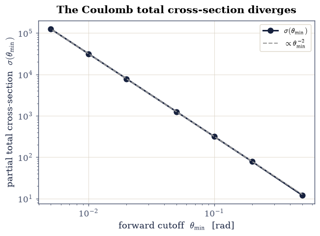
Fig. 144 The Coulomb total cross-section diverges (\(E=1\), \(k=1\)): the partial total \(\sigma(\theta_{\min})=\int_{\theta_{\min}}^{\pi}(d\sigma/d\Omega)\,2\pi\sin\theta\,d\theta\) grows without bound as the forward cutoff \(\theta_{\min}\to0\) (log-log axes; the dashed guide is the \(\propto\theta_{\min}^{-2}\) small-angle scaling). The divergence is the signature of the infinite-range \(1/r\) force; physical screening at large distance supplies the cutoff that makes a real total cross-section finite.

small-angle limit at b=8.0: numeric θ = 0.12475, k/(Eb) = 0.12500  (rel.err 0.20%)

Validation 7 — the total cross-section diverges, and \(\theta\approx k/(Eb)\)

Two checks. First, the partial total cross-section strictly increases as the forward cutoff \(\theta_{\min}\) shrinks: the Coulomb total has no finite limit. Second, the large-\(b\) small-angle limit \(\theta\approx k/(Eb)\) holds against a measured trajectory (the \(4\%\) tolerance covers the finite-distance systematic, which is largest exactly here, at the widest \(b\)).

✓  the Coulomb total cross-section diverges (infinite range)   [σ grows 10432× as θ_min: 0.5→0.005]
✓  small-angle deflection follows θ ≈ k/(Eb) for large b   [got 0.124754 vs expected 0.125 (rtol=0.04, atol=1e-09)]

True

Notebook summary

• The scattering geometry and single trajectories integrated through a repulsive potential; the deflection angle as a function of impact parameter.

• The differential cross-section assembled from \(d\sigma/d\Omega=(b/\sin\theta)|db/d\theta|\), reproducing the Rutherford \(1/\sin^4(\theta/2)\) law; attractive versus repulsive scattering; and the small-angle divergence of the total cross-section for the Coulomb tail.

Outlook

• Screened Coulomb (Yukawa). \(V(r)=k\,e^{-r/a}/r\) cuts off the force beyond the screening length \(a\), giving a finite total cross-section; integrate \(\theta(b)\) numerically and watch the small-angle divergence tamed.

• Rainbow and glory angles. An attractive potential with a softer core can make \(d\theta/db\) vanish at some \(b\) (\(db/d\theta\to\infty\) in Eq. 156), a rainbow singularity in \(d\sigma/d\Omega\), the classical analogue of the optical rainbow; \(\theta\to0\) or \(\pi\) at nonzero \(b\) gives a glory.

• Hard-sphere scattering. The analytic warm-up: a rigid sphere of radius \(R\) gives the isotropic \(d\sigma/d\Omega=R^2/4\) and finite total \(\sigma=\pi R^2\): the geometric cross-section, with no forward divergence.

• The quantum cross-section. The Born approximation for the Coulomb potential reproduces the Rutherford formula exactly: a striking classical/quantum agreement we return to in Volume VI.

References

[GPS02]

Herbert Goldstein, Charles P. Poole, and John L. Safko. Classical Mechanics. Pearson, 3 edition, 2002.

[LL76] (1,2)

L. D. Landau and E. M. Lifshitz. Mechanics. Volume 1 of Course of Theoretical Physics. Butterworth–Heinemann, 3 edition, 1976.

[Nol16]

Wolfgang Nolting. Theoretical Physics 2: Analytical Mechanics. Springer, 2016.

Take this notebook with you

Use the download button (↓) in the toolbar above to save this notebook and run it yourself. The published notebooks ship without worked solutions; if you would like the reference solutions — to teach from or to check your own work — get in touch: hello@ramador.me.