


6.27 Quantum Information: Gates, Circuits, Teleportation, and Algorithms#
Notebook overview#
This is the capstone of Volume VI, and its argument is a single realization: a quantum computer is nothing more than the linear algebra this volume has been doing all along. A qubit is the two-state system of Movement I (§6.4, §6.8); a quantum gate is a unitary matrix (the evolution of §6.7); a quantum circuit is a product of gates acting on a tensor-product state (§6.14, §6.8); a measurement is the Born rule (§6.5). Nothing new is required — only these pieces, arranged deliberately.
From them, and from entanglement as a resource (§6.25, §6.26), come feats with no classical analogue. Quantum teleportation transfers an unknown qubit across space using only a shared Bell pair and two classical bits — reproducing the input exactly, for every measurement outcome, without ever cloning it (the no-cloning theorem, itself a one-line consequence of linearity). Quantum algorithms turn superposition and interference into speed: Deutsch–Jozsa decides a global property of a function in a single query where classical computation may need exponentially many; Grover’s search finds a marked item among \(N\) in about \(\tfrac\pi4\sqrt N\) steps by amplitude amplification — a rotation in a 2-D subspace, the same geometry we have used throughout. Shor’s algorithm (named, not built) would factor large integers efficiently, breaking the cryptography that secures the internet — the reason quantum computing commands the attention it does. And the density matrix and entropy of §6.26 are exactly the tools that quantify the entanglement these protocols spend and the decoherence that quantum error correction must fight.
We build every runnable, validated result from scratch in NumPy — gates as
unitary matrices, circuits as @ products of numpy.kron tensor factors,
measurement by Born-rule sampling. The professional software (Qiskit) appears only
as an illustration, explicitly fenced so it never enters the numerical spine.
The Qiskit fence. The runnable, validated core is entirely from-scratch NumPy. Qiskit appears once, in a display-only cell (an import guarded so it cannot fail the build), purely to show that the industry notation is a shorthand for the matrices we build by hand:
His the Hadamard gate,cxis our CNOT,numpy.kronis the tensor product. The physics is the linear algebra, not the library.
Method specificity. Gates are unitary matrices; multi-qubit gates and states use
numpy.kron; controlled gates are built from projectors \(P_0\otimes I+P_1 \otimes U\); circuits are@products; measurement is Born-rule sampling withnumpy.random.default_rng.
Theory in brief#
The qubit and the state of many qubits#
A qubit is a normalized vector in \(\mathbb C^2\) (§6.4, §6.8). \(n\) qubits live in
the tensor product \((\mathbb C^2)^{\otimes n}\) of dimension \(2^n\) (numpy.kron);
that exponential growth is the root of quantum computing’s power — and of the cost
of simulating it classically.
Quantum gates as unitaries#
A gate is a unitary matrix (norm-preserving, so probability is conserved — the evolution of §6.7). Single-qubit: the Paulis \(X,Y,Z\) (§6.6), the Hadamard \(H\) (which makes superposition, \(H|0\rangle=(|0\rangle+|1\rangle)/\sqrt2\)), the phase gates \(S,T\). Multi-qubit: the CNOT, built from projectors,
which flips the target iff the control is \(|1\rangle\); controlled-\(U\) and the Toffoli generalize it. A small set (e.g. \(H,T,\mathrm{CNOT}\)) is universal — it approximates any unitary (named, not proved).
Quantum circuits and measurement#
A circuit is a product of unitary matrices (read right to left), gates on disjoint qubits combined by tensor product (\(I\) on untouched wires):
The Bell state is three symbols: from \(|00\rangle\), apply \(H\) to qubit 0, then \(\mathrm{CNOT}(0,1)\), giving \((|00\rangle+|11\rangle)/\sqrt2\) (the §6.8 Bell state). Measurement is the Born rule (§6.5): outcome probabilities are squared amplitudes, and repeated runs are Born-rule sampling (§6.4).
The no-cloning theorem#
No unitary copies an arbitrary unknown qubit:
a one-line consequence of linearity — a cloner that works on \(|0\rangle\) and \(|1\rangle\) fails on their superposition. This is why quantum information cannot be copied, why teleportation must move rather than copy, and why eavesdropping is detectable.
Quantum teleportation#
Alice holds an unknown \(|\psi\rangle\) and shares a Bell pair with Bob. She applies \(\mathrm{CNOT}\) then \(H\) to her two qubits, measures them (two classical bits), and sends the bits to Bob, who applies a Pauli correction to recover \(|\psi\rangle\) exactly:
No clone is made (Alice’s copy is destroyed by measurement), nothing travels faster than light (Bob needs the bits), yet the unknown state is transferred — entanglement plus classical communication as a channel. Its dual, superdense coding (Eq. 649), sends two classical bits by transmitting one qubit of a shared pair.
Quantum parallelism, and two algorithms#
A unitary applied to a superposition acts on all basis states “at once” (parallelism), but a measurement returns only one — so the art of a quantum algorithm is to arrange interference that concentrates amplitude on the answer.
Deutsch–Jozsa (Eq. 651): given \(f\) promised constant or balanced, a superposition of all inputs, the oracle (a phase kickback), and a second layer of Hadamards make the all-zeros outcome certain iff \(f\) is constant — one query where classical needs up to \(2^{n-1}+1\).
Grover (Eq. 652): to find a marked item among \(N=2^n\), each iteration applies the oracle (sign-flip the marked amplitude) then the diffuser (reflection about the mean), which together rotate the state toward the marked item in the 2-D marked/unmarked plane. After \(\sim\tfrac\pi4\sqrt N\) iterations the amplitude concentrates on the answer.
Shor, error correction, and why this matters#
Shor’s algorithm (Eq. 653) factors an \(n\)-bit integer in polynomial time by using the quantum Fourier transform to find a period — breaking RSA. Its number theory is a horizon; its significance is the punchline. And decoherence (§6.26) is the central obstacle, so real machines need quantum error correction — encoding one logical qubit in many physical ones — the entanglement and entropy of §6.26 being exactly its tools.
Reference: Nielsen & Chuang [NC10] (the standard text — gates, circuits, teleportation, Deutsch–Jozsa, Grover, Shor); Griffiths [GS18]; Preskill’s lecture notes. Cross-reference §6.4/§6.8 (the qubit, the Bloch sphere, the Bell state, Born-rule sampling), §6.5 (measurement), §6.6 (Pauli operators), §6.7 (unitary evolution), §6.14 (tensor products), §6.25 (Bell nonlocality — the resource certified), §6.26 (density matrix, entropy, decoherence), and — as the volume’s closer — §6.1–§6.3 (the linear-algebra arsenal now revealed as the machinery of quantum computation), forward to Volume VII. Named as horizons: Shor’s algorithm, quantum error correction, physical qubit implementations, the universality proofs.
Setup#
Everything runnable is from-scratch NumPy. The data are the conventions and the gate
alphabet: qubit 0 is the leftmost (most-significant) tensor factor, so an \(n\)-qubit state
is a length-\(2^n\) vector indexed by the integer \(b_0b_1\cdots b_{n-1}\); circuits are @
products read right to left; and the fixed specimens every circuit below is written in
terms of are the single-qubit matrices \(I,X,Y,Z,H,S,T\), the projectors \(P_0=|0\rangle
\langle0|\) and \(P_1=|1\rangle\langle1|\) they get combined with, and the computational-basis
kets \(|0\rangle,|1\rangle\). The instruments are the register plumbing and the meters:
kron_list folds numpy.kron over a list, single(U, q, nq) pads a one-qubit gate with
identities on the untouched wires (\(I\otimes\cdots\otimes U\otimes\cdots\otimes I\)),
basis_state assembles a basis ket from a bit string, is_unitary is the admission test
\(U^\dagger U=I\), and born_probabilities/sample_measurements read outcome statistics off
a state vector by the Born rule of §6.5 and the numpy.random.default_rng
sampling of §6.4. The multi-qubit construction this notebook is
named for is deliberately absent: you write the projector sum controlled and its
two-control generalization toffoli in Exercise 2, and every circuit, protocol and
algorithm after that is assembled in the exercise that needs it.
The Setup below holds this notebook’s data and instruments — nothing you are asked to build. It is collapsed so the building stays yours; expand it whenever you want the details.
Exercise 1 — Single-qubit gates as unitaries#
A quantum gate is nothing more exotic than a unitary matrix, and the single-qubit alphabet fits on one line each: the Paulis \(X,Y,Z\) — the observables of §6.6, now read as operations rather than as questions — the Hadamard \(H\), and the phase gates \(S=\mathrm{diag}(1,i)\) and \(T=\mathrm{diag}(1,e^{i\pi/4})\) that rotate about the polar axis by a quarter and an eighth turn. Unitarity, \(U^\dagger U=I\), is the only admission requirement quantum mechanics imposes: it is what keeps the total probability at one, and it is why a gate is the same object as the time evolution of §6.7, packaged into a single step. Two identities fix the Hadamard’s character — \(H|0\rangle=(|0\rangle+|1\rangle)/\sqrt2\), so it manufactures superposition from a definite state, and \(H^2=I\), so applying it twice undoes it.
Take the matrices
X,Y,Z,H,S,Tfrom the setup and collect them by name.Verify each is unitary (\(U^\dagger U=I\)) with the setup’s
is_unitary.Show \(H|0\rangle=(|0\rangle+|1\rangle)/\sqrt2\) and \(H^2=I\).
Note the Paulis are the §6.6 observables and that gates are the unitary evolution of §6.7, packaged.
  X: unitary = True
  Y: unitary = True
  Z: unitary = True
  H: unitary = True
  S: unitary = True
  T: unitary = True
H|0⟩ = [0.7071+0.j 0.7071+0.j]   = (|0⟩+|1⟩)/√2: True
H² = I: True
Validation 1#
Every gate must be unitary, and the Hadamard must create an equal superposition from \(|0\rangle\) (with \(H^2=I\)): quantum gates are unitary matrices.
✓ quantum gates are unitary matrices; H creates an equal superposition
True
Exercise 2 — Multi-qubit gates and the CNOT#
One gate separates a quantum computer from a pile of independent qubits: a controlled
gate, which acts on one wire only when another wire says so. Its matrix is written with the
projectors \(P_0=|0\rangle\langle0|\) and \(P_1=|1\rangle\langle1|\), which resolve the control
qubit into its two branches — the target is left alone in the \(|0\rangle\) branch and acted on
by \(U\) in the \(|1\rangle\) branch — so the whole gate is the two-term sum \(P_0\otimes I+P_1
\otimes U\) Eq. 645. On a register of \(n_q\) qubits each term is a numpy.kron chain
carrying the projector on the control wire, \(I\) or \(U\) on the target, and \(I\) on every wire
that is neither, which is what makes one expression valid for any control/target pair. With
\(U=X\) this is the CNOT, classical XOR made reversible: \(|00\rangle\to|00\rangle\),
\(|01\rangle\to|01\rangle\), \(|10\rangle\to|11\rangle\), \(|11\rangle\to|10\rangle\). A second
control gives the Toffoli (CCX), a sum over the four combinations \((P_0\text{ or }P_1)\)
on one control and \((P_0\text{ or }P_1)\) on the other, with \(X\) on the target in exactly the
one term where both controls are \(|1\rangle\). The Toffoli is universal for classical
reversible logic — which is how ordinary computation embeds inside unitary evolution.
Write
controlled(U, ctrl, tgt, nq), returning the two-term projector sum above embedded on annq-qubit register (identities on every other wire), and form the CNOT ascontrolled(X, ctrl=0, tgt=1, nq=2). Write this one yourself — the implementation is the lesson.Verify it is unitary.
Confirm the truth table: \(\mathrm{CNOT}|00\rangle=|00\rangle\), \(\mathrm{CNOT} |10\rangle=|11\rangle\), and so on.
Write
toffoli(c1, c2, tgt, nq)as the four-term sum described above, and check that it flips the target on \(|110\rangle\) and is unitary. Write this one yourself — the implementation is the lesson.
Cite Eq. 645.
CNOT unitary: True
  CNOT|00⟩ = |00⟩
  CNOT|01⟩ = |01⟩
  CNOT|10⟩ = |11⟩
  CNOT|11⟩ = |10⟩
Toffoli|110⟩ = |111⟩ (flips target iff both controls are 1); unitary: True
Validation 2#
The CNOT must be unitary and flip the target iff the control is \(|1\rangle\) (\(|00\rangle\to|00\rangle\), \(|10\rangle\to|11\rangle\)): controlled gates entangle qubits.
✓ CNOT is unitary and flips the target iff the control is |1⟩ (controlled gates entangle)
True
Exercise 3 — Circuits and the Bell state#
A circuit is a product of unitary matrices Eq. 646, and because a matrix acts on the vector to its right the product is read right to left: the gate applied first stands last. Three symbols are then enough for the most famous state in the subject. Starting from \(|00\rangle\), a Hadamard on qubit 0 — embedded as \(H\otimes I\), since qubit 1 is untouched — gives \((|00\rangle+|10\rangle)/\sqrt2\); a CNOT controlled by qubit 0 flips qubit 1 in the second term only, and the result is \((|00\rangle+|11\rangle)/\sqrt2\). That is the Bell state of §6.8, whose random marginals and perfect correlations the volume has already met — here manufactured to order by \(\mathrm{CNOT}\,(H\otimes I)\).
Start from \(|00\rangle\) with the setup’s
basis_state.Apply \(H\) to qubit 0, embedded as \(H\otimes I\) by the setup’s
single.Apply the
controlledCNOT you wrote in Exercise 2.Confirm the output is \((|00\rangle+|11\rangle)/\sqrt2\) — the Bell state of §6.8.
Cite Eq. 646.
Bell circuit output: [0.7071 0.     0.     0.7071]
matches §6.8 Bell state: True
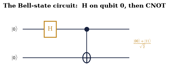
Fig. 603 The entanglement of the whole movement, in three gates. The circuit reads left to right: qubit 0 (top) gets a Hadamard, making \((|0\rangle+|1\rangle)/\sqrt2\); then a CNOT (control ● on qubit 0, target ⊕ on qubit 1) flips qubit 1 exactly when qubit 0 is \(|1\rangle\). The output is \((|00\rangle+|11\rangle)/\sqrt2\) — the Bell state of §6.8, whose random marginals (§6.25) and maximally mixed reduced state (§6.26) this course has now fully explained. A quantum circuit is a product of unitary matrices; this one is \(\mathrm{CNOT}\,(H\otimes I)\).#
Validation 3#
The \(H+\mathrm{CNOT}\) circuit must prepare exactly the Bell state \((|00\rangle+ |11\rangle)/\sqrt2\) of §6.8.
✓ the H + CNOT circuit prepares the §6.8 Bell state [max|Δ| = 0 (rtol=1e-09, atol=1e-09)]
True
Exercise 4 — Measurement and Born sampling#
A state vector is not what a machine reports. What comes back from a real device is a list of
shots, each one an outcome drawn at random with the Born probability
\(|\langle x|\Psi\rangle|^2\) (§6.5), and the distribution has to be
reconstructed from the counts (§6.4). For the Bell state
\((|00\rangle+|11\rangle)/\sqrt2\) the exact probabilities are \(\tfrac12\) on \(00\), \(\tfrac12\) on
\(11\), and zero on \(01\) and \(10\): the two qubits are perfectly correlated, so measuring one
fixes the other — the very correlation the Bell test of §6.25 turned
into a violated inequality. Five thousand shots from a numpy.random.default_rng(2718)
generator are enough to see it, sampling noise included.
Compute the outcome probabilities as squared amplitudes with the setup’s
born_probabilities(§6.5).Sample 5000 shots with the setup’s
sample_measurementsand a seedednumpy.random.default_rng(§6.4).Histogram the outcomes.
Confirm only \(00\) and \(11\) appear, each about half the time (perfect correlation).
Cite Eq. 646.
Born probabilities: [0.5 0.  0.  0.5]
  00:  2508  (50.2%)
  01:     0  (0.0%)
  10:     0  (0.0%)
  11:  2492  (49.8%)
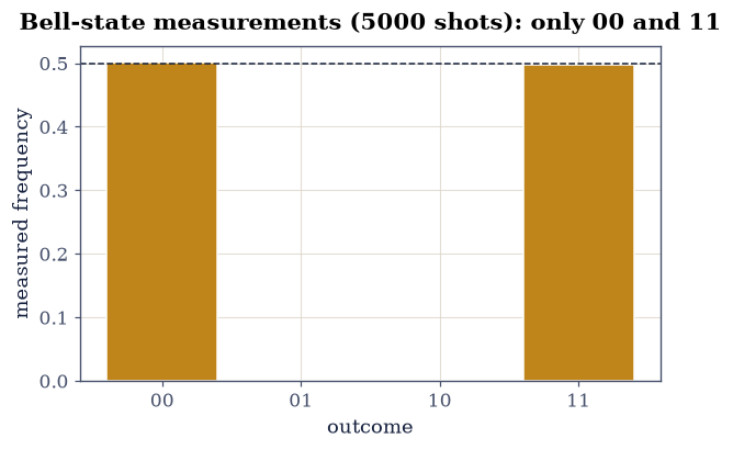
Fig. 604 Measurement is the Born rule, sampled. Five thousand measurements of the Bell state \((|00\rangle+|11\rangle)/\sqrt2\) give only the outcomes \(00\) and \(11\), each about half the time (amber); \(01\) and \(10\) never occur. The two qubits are perfectly correlated — measuring one fixes the other — which is precisely the correlation the Bell test (§6.25) turned into a violated inequality. Repeated runs of a circuit reveal its output distribution, one shot at a time, exactly as a real quantum computer reports its results.#
Validation 4#
Sampled Bell-state measurements must give only \(00\) and \(11\), each near 50% — the Born rule in action.
✓ sampled Bell measurements give only 00 and 11 with equal frequency (Born rule)
True
Exercise 5 — The no-cloning theorem#
No unitary copies an arbitrary unknown qubit Eq. 647, and the obstruction is not dynamical but a single line of linearity. Suppose some \(U\) cloned, so that \(U|\psi\rangle|0\rangle=|\psi\rangle|\psi\rangle\) for every \(|\psi\rangle\). Demanding it on the two basis states fixes \(U|00\rangle=|00\rangle\) and \(U|10\rangle=|11\rangle\) — which is exactly the CNOT of Exercise 2. Linearity then leaves no freedom on a superposition: feeding it \(|+\rangle|0\rangle\) with \(|+\rangle=(|0\rangle+|1\rangle)/\sqrt2\) must give \((|00\rangle+|11\rangle)/\sqrt2\), the entangled Bell state, whereas a genuine clone would have to produce the product \(|+\rangle|+\rangle\). The two are different vectors, so no such \(U\) exists. This is why quantum information cannot be duplicated, why teleportation has to move a state rather than copy it, and why an eavesdropper cannot listen undetected.
Build the hypothetical basis cloner as the CNOT you wrote in Exercise 2 — the unitary that does copy \(|0\rangle\) and \(|1\rangle\).
Apply it to \(|+\rangle|0\rangle\).
Compare the result with the product \(|+\rangle|+\rangle\) a true clone would give.
Conclude cloning is impossible — the reason teleportation must move, not copy.
Cite Eq. 647.
cloner on |+⟩|0⟩ = [0.707 0.    0.    0.707]
a true clone |+⟩|+⟩ = [0.5 0.5 0.5 0.5]
equal? False  → cloning the superposition FAILS
Validation 5#
A hypothetical cloner fixed to copy \(|0\rangle\) and \(|1\rangle\) must fail on their superposition (\((|00\rangle+|11\rangle)/\sqrt2\ne|+\rangle|+\rangle\)): unknown quantum states cannot be cloned.
✓ a cloner consistent on |0⟩,|1⟩ fails on their superposition — unknown states cannot be cloned
True
Exercise 6 — Quantum teleportation#
Alice holds one qubit in an unknown state \(|\psi\rangle\) and shares a Bell pair with Bob, who is far away; the three qubits together are the vector \(|\psi\rangle\otimes(|00\rangle+ |11\rangle)/\sqrt2\) in \(\mathbb C^8\). Alice applies \(\mathrm{CNOT}(0,1)\) and then \(H\) on qubit 0, which rewrites that vector as a sum of four equally weighted branches, one for each value of the two bits she is about to read. Measuring her two qubits selects a branch — the projector \(P_{m_0}\otimes P_{m_1}\otimes I\), renormalized — and in each branch Bob’s qubit is \(|\psi\rangle\) up to one Pauli, so the two classical bits \((m_0,m_1)\) tell him which of \(I,X,Z,ZX\) to undo: \(Z^{m_0}X^{m_1}\) Eq. 648. The fidelity \(|\langle\psi|\text{Bob}\rangle|^2\) is then exactly 1 for every outcome, each occurring with probability \(\tfrac14\). Nothing is cloned — Alice’s copy is destroyed by her measurement, consistent with Exercise 5 — and nothing outruns light, because without the two bits Bob’s qubit is maximally mixed. The specimen state is \(|\psi\rangle=\cos(0.7)|0\rangle+ e^{1.1i}\sin(0.7)|1\rangle\), chosen complex so that a real-valued accident cannot flatter us.
Write
teleport(psi): form the three-qubit state, apply Alice’s \(\mathrm{CNOT}(0,1)\) and \(H(0)\) with your Exercise 2controlledand the setup’ssingle, project onto each of the four outcomes \((m_0,m_1)\) and renormalize, read off Bob’s qubit, apply the correction \(Z^{m_0}X^{m_1}\), and return the branch probability, the fidelity and the correction’s name for each outcome. Write this one yourself — the implementation is the lesson.Run it on the unknown \(|\psi\rangle\) above.
Confirm the fidelity is 1 for all four outcomes, with the corrections \(I,X,Z,ZX\) and probability \(\tfrac14\) each.
Note what the protocol spends: one entangled pair and two classical bits per qubit sent.
Cite Eq. 648.
  outcome (0,0): prob=0.250  correction=II  fidelity=1.000000
  outcome (0,1): prob=0.250  correction=IX  fidelity=1.000000
  outcome (1,0): prob=0.250  correction=ZI  fidelity=1.000000
  outcome (1,1): prob=0.250  correction=ZX  fidelity=1.000000
teleportation recovers the unknown state exactly for all four outcomes
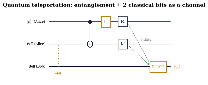
Fig. 605 Moving the uncopyable. Alice’s unknown qubit \(|\psi\rangle\) (top) and a shared Bell pair (middle/bottom, the wavy link) are the input. Alice applies CNOT then H to her two qubits and measures them (the meters), producing two classical bits (double lines) that she sends to Bob. Bob applies the Pauli correction \(Z^{m_0}X^{m_1}\) — one of \(I,X,Z,ZX\) — and his qubit becomes \(|\psi\rangle\) exactly. No copy was made (measurement destroyed Alice’s), and nothing outran light (Bob needed the classical bits); yet the unknown state crossed the gap, carried by one ebit of entanglement (§6.26) and two classical bits.#
Validation 6#
The teleported state must match the input with fidelity 1 for all four measurement outcomes, using the corrections \(I,X,Z,ZX\): teleportation transfers an unknown qubit via one Bell pair and two classical bits.
✓ teleportation transfers an unknown qubit exactly for all outcomes (corrections I/X/Z/ZX)
True
Exercise 7 — Deutsch–Jozsa#
A function \(f:\{0,1\}^n\to\{0,1\}\) is promised to be either constant or balanced (equal to 0 on exactly half its inputs). Classically the promise is worth little: in the worst case one must evaluate \(f\) on \(2^{n-1}+1\) inputs before the answer is certain. One quantum query settles it Eq. 651. The oracle is the reversible embedding \(U_f:|x\rangle|y\rangle\to|x\rangle|y\oplus f(x)\rangle\), a permutation matrix with a single 1 in each column, and it is queried on a superposition of all inputs Eq. 650. Preparing the ancilla in \(|1\rangle\) before the Hadamards puts it in \((|0\rangle-|1\rangle)/\sqrt2\), an eigenvector of the XOR, so the oracle’s action shows up as a phase kickback \((-1)^{f(x)}\) on the input register instead of a change in the ancilla. A constant \(f\) contributes a global sign that a second layer of Hadamards folds back onto \(|0\cdots0\rangle\) with certainty; a balanced \(f\) makes those phases cancel there exactly, so the all-zeros amplitude vanishes. The answer is therefore not “a value of \(f\)” but a global property of it, read off in one shot. Four oracles on \(n=3\) make the test: \(f\equiv0\) and \(f\equiv1\) (constant), and the parity of \(x\) and its lowest bit (balanced).
Write
deutsch_jozsa(f, n): build \(U_f\) on \(n+1\) qubits, prepare \(|0\rangle^{\otimes n}|1\rangle\), apply Hadamards to every qubit, apply \(U_f\), apply Hadamards to the input register, and return"constant"or"balanced"from the probability of an all-zeros input register. Write this one yourself — the implementation is the lesson.Run it on the two constant and the two balanced oracles above.
Confirm the verdict is right in every case, from a single oracle query.
Compare with the classical worst case, \(2^{n-1}+1\) evaluations.
  f ≡ 0 (constant)         → constant  (expected constant)
  f ≡ 1 (constant)         → constant  (expected constant)
  parity (balanced)        → balanced  (expected balanced)
  first bit (balanced)     → balanced  (expected balanced)
one query decided each; classical worst case needs up to 2^(n-1)+1 = 5
Validation 7#
Deutsch–Jozsa must return ‘constant’ for the constant oracles and ‘balanced’ for the balanced ones, each in a single query.
✓ Deutsch–Jozsa decides the global property (constant vs balanced) with a single evaluation
True
Exercise 8 — Grover’s search#
Searching an unstructured list of \(N=2^n\) items classically costs \(\sim N/2\) queries; Grover’s algorithm needs about \(\tfrac\pi4\sqrt N\) Eq. 652, and the reason is geometry. Two reflections make the iteration: the oracle, which flips the sign of the marked amplitude alone (the identity with a single \(-1\) on the diagonal), and the diffuser \(2|s\rangle\langle s|-I\), a reflection about the uniform state \(|s\rangle=H^{\otimes n} |0\rangle\) — equivalently, about the mean amplitude. A reflection followed by a reflection is a rotation, and here it happens in the two-dimensional plane spanned by the marked state and the uniform superposition of the rest, turning the state by a fixed angle \(2\theta\) with \(\theta=\arcsin(1/\sqrt N)\) per iteration. Starting at angle \(\theta\) from the unmarked axis, the state reaches the marked axis after \((\pi/2-\theta)/2\theta\approx\tfrac\pi4\sqrt N\) steps. That the answer is a rotation carries a practical warning: keep iterating past the optimum and the state rotates straight past the answer, so the success probability falls again — visible if the \(N=64\) case is run for 16 iterations instead of the optimal 6.
Write
grover(marked, n, n_iter=None): start from \(|s\rangle\), apply the oracle then the diffusern_itertimes (defaulting to the exact optimum \(\mathrm{round}\big((\pi/2-\theta)/2\theta\big)\)), and return the final marked probability together with its history over the iterations. Write this one yourself — the implementation is the lesson.Run it at the optimal iteration count for \(n=2,\dots,8\) and confirm the marked probability is near 1 throughout.
Take the history for \(N=64\) well past the optimum and see the overshoot.
Read each iteration as a rotation toward the marked state in the 2-D marked/unmarked plane.
Cite Eq. 652.
Grover success probability at the optimal iteration count:
  N =   4:  P(marked) = 1.0000  (~(π/4)√N iterations)
  N =   8:  P(marked) = 0.9453  (~(π/4)√N iterations)
  N =  16:  P(marked) = 0.9613  (~(π/4)√N iterations)
  N =  32:  P(marked) = 0.9992  (~(π/4)√N iterations)
  N =  64:  P(marked) = 0.9966  (~(π/4)√N iterations)
  N = 128:  P(marked) = 0.9956  (~(π/4)√N iterations)
N = 256: P(marked) = 0.9999 (~(π/4)√N iterations)
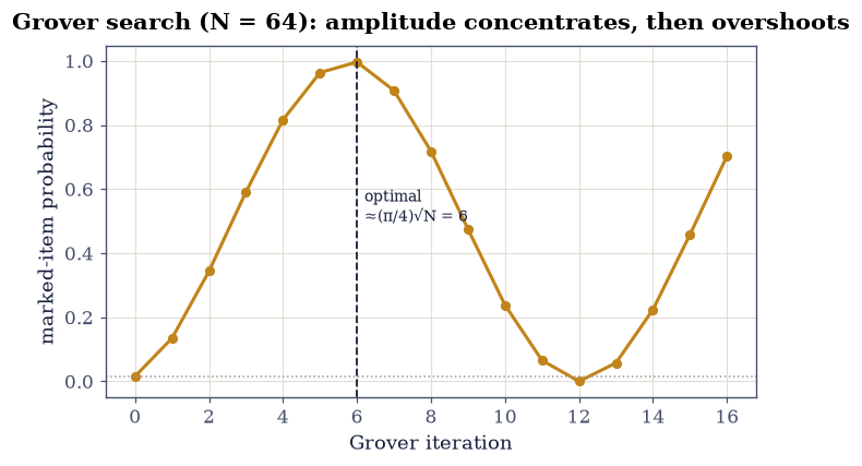
Fig. 606 Amplitude amplification is a rotation. For \(N=64\) items, the marked item’s probability (amber) starts at \(1/N\approx1.6\%\) and climbs with each Grover iteration, reaching \(\approx99.7\%\) at the optimal step (dashed, \(\lfloor\tfrac\pi4\sqrt N\rfloor=6\)). Each iteration rotates the state by a fixed angle in the 2-D plane spanned by the marked and unmarked states — the same rotation geometry this volume has used from spin to the Bloch sphere — so running too long overshoots and the probability falls again. The quadratic speedup (\(\sqrt N\) vs \(N/2\)) is provably optimal for unstructured search.#
Validation 8#
Grover must find the marked item with high probability in about \(\tfrac\pi4\sqrt N\) iterations, for \(N\) up to 256: amplitude amplification gives a quadratic speedup.
✓ Grover finds the marked item with probability >0.9 in ~(π/4)√N iterations (N up to 256)
True
Exercise 9 — The Qiskit fence: same circuit, professional notation (student)#
The professional software the field runs on writes the Bell circuit in three lines, and it is
worth seeing exactly what those lines stand for. Qiskit’s qc.h(0) is our \(H\otimes I\) —
the setup’s single(H, 0, 2); its qc.cx(0, 1) is our CNOT, the projector sum
controlled(X, 0, 1, 2) of Exercise 2; and the tensor product that assembles a two-qubit
register is numpy.kron. The library is a notation, not a physics. To keep that claim
honest this notebook never lets it into the numerical spine: the Qiskit call below is
display-only and guarded, so an absent installation prints a message and changes nothing,
while the validated Bell state is the one the from-scratch matrices compute.
Read the Qiskit rendering of the Bell circuit below (it is not part of the validated computation).
Rebuild the same circuit from the matrices —
controlled(X, 0, 1, 2)andsingle(H, 0, 2)onbasis_state("00")— and compare it with the Exercise 3 result.Note the correspondence:
h(0)is our \(H\otimes I\),cx(0,1)is our CNOT (\(P_0\otimes I+P_1\otimes X\)), and Qiskit’s tensor product isnumpy.kron.Conclude that the library is a convenient notation; the physics is the linear algebra we already command.
Cite Eq. 646.
The Qiskit rendering (pin qiskit~=2.0), shown for reference only:
from qiskit import QuantumCircuit          # display-only; not run in this build
qc = QuantumCircuit(2)
qc.h(0)                                    # our  single(H, 0, 2)
qc.cx(0, 1)                                # our  controlled(X, 0, 1, 2)
print(qc.draw())                           # the same H + CNOT circuit as Fig. 1
Qiskit not installed — and it does not matter: the from-scratch NumPy
matrices above computed and validated the Bell state. Qiskit's h(0)/cx(0,1)
are exactly our single(H,0,2) and controlled(X,0,1,2). (pip install 'qiskit~=2.0')

from-scratch Bell state still correct: True
Validation 9#
The check depends only on the from-scratch NumPy: our matrices reproduce the Bell circuit, confirming the professional tools are shorthand for the operations we built here.
✓ the from-scratch matrix circuit reproduces the Bell state (the tools are shorthand for these operations) [max|Δ| = 0 (rtol=1e-09, atol=1e-09)]
True
Exercise 10 — Entanglement as a resource: entropy across a protocol (student / challenge)#
Entanglement is not a mood a state is in; it is a quantity that gets spent, and §6.26 already supplies the meter. Trace one half out of the Bell pair and what is left is the maximally mixed single-qubit state \(\tfrac12 I\), whose von Neumann entropy \(-\sum_k\lambda_k\log_2\lambda_k\) is exactly 1 bit — one ebit, the standard unit of the resource. Teleportation consumes one of them per qubit sent: after Alice’s measurement the pair is gone, and a second teleportation needs a second pair. Written as a ledger, Eq. 654 and Eq. 649 say one ebit plus two classical bits buys the transfer of one qubit, and the dual protocol spends one ebit plus one qubit to buy two classical bits. The same ledger explains why real machines are hard: decoherence (§6.26) leaks this resource to the environment for free, which is what quantum error correction exists to fight.
Restate the §6.26 partial trace and von Neumann entropy as the two tools you need, and apply them to the Bell pair’s density matrix.
Confirm the reduced state carries \(S=1\) bit — one ebit.
Conclude teleportation costs exactly one ebit plus two classical bits per qubit sent.
Connect to decoherence (§6.26): real devices leak this resource to the environment, which is why they need quantum error correction.
Cite Eq. 654.
entanglement entropy of the shared Bell pair: S(ρ_A) = 1.000000 bit = 1 ebit
teleportation consumes exactly this one ebit (+ 2 classical bits) to send one qubit
decoherence (§6.26) leaks such entanglement to the environment — why QEC is needed
Validation 10#
The shared Bell pair must carry exactly one bit of entanglement entropy (one ebit) — the resource teleportation spends, measured with the tools of §6.26.
✓ teleportation consumes one bit of entanglement (one ebit) [got 1 vs expected 1 (rtol=1e-06, atol=1e-06)]
True
Exercise 11 — A small algorithm, end to end (challenge / stretch)#
Nothing new is needed for a complete computation — the pieces are all in hand, and the point
of this last exercise is that they compose. Take \(n=3\), so \(N=8\) items, and mark
\(|101\rangle\), index 5 in the length-8 state vector. The uniform superposition is the start,
the optimal iteration count from Exercise 8 is
\(\mathrm{round}\big((\pi/2-\theta)/2\theta\big)=2\) for \(N=8\), and the final state is read the
way a device would report it: 4000 shots sampled from the Born distribution with a seeded
numpy.random.default_rng, not a probability printed off the amplitudes. If the marked item
dominates those counts, then a from-scratch NumPy toolkit — matrices, numpy.kron, @ — has
just run a quantum algorithm end to end.
Choose \(n=3\) (\(N=8\)) and the marked item \(|101\rangle\) (index 5), and take the success probability from your Exercise 8
grover.Rebuild the final state vector explicitly: uniform superposition, then the optimal number of oracle+diffuser iterations.
Sample 4000 shots of it with the setup’s
sample_measurementsand a seedednumpy.random.default_rng.Confirm the marked item dominates the measured counts — a working quantum algorithm assembled entirely from the toolkit.
3-qubit Grover for |101⟩ (index 5): 2 iterations, P(marked) = 0.9453
most-sampled outcome: |101⟩ (95.1% of shots) — the marked item
Validation 11#
The assembled 3-qubit Grover circuit must return the marked item \(|101\rangle\) as its dominant measured outcome: the from-scratch toolkit composes into working quantum algorithms.
✓ the assembled from-scratch algorithm solves its stated problem (Grover finds |101⟩)
True
Exercise 12 — (Synthesis) The volume, closed#
The course began with a two-state system — an electron’s spin, a single qubit — and the modest claim that quantum mechanics is linear algebra. It ends here with that same qubit, that same linear algebra, assembled into a machine that teleports states it cannot copy and searches faster than any classical computer can. Nothing new was needed. Gates are the unitary evolution we studied in Movement I (§6.7); circuits are their products on the tensor-product spaces of §6.14; measurement is the Born rule of §6.5; entanglement is the correlation we measured in the Bell tests of §6.25 and quantified with the entropy of §6.26; and the professional software is a shorthand for the matrices we built by hand. The arsenal of §6.1–§6.3 — vectors, inner products, Hermitian and unitary matrices, eigenvalues — turns out to have been the machinery of quantum computation all along.
It is a strange and beautiful thing that the rules we inferred from spectral lines and Stern–Gerlach beams describe a computer. We did not add anything to quantum mechanics to get here; we only asked what it could do if we arranged the interference on purpose. The answer — a machine that breaks codes and moves the uncopyable — was hiding in the linear algebra from the first page. And the same decoherence that made a superposition look classical (§6.26) is the dragon that quantum engineering must slay: every protocol here assumes coherence the real world is always trying to take away, which is why quantum error correction, built from the very entanglement and entropy we have used, is the central challenge of the field.
Volume VI is complete — from the postulates to the atom, from the three faces of approximation to the foundations, and now to the information the theory can carry. Volume VII takes the density matrix we just used and gives it a temperature, \(\rho=e^{-\beta H}/Z\): quantum statistical mechanics, where the quantum world meets the thermodynamic one, and the linear algebra of the very small becomes the physics of the very many.
Notebook summary#
Gates and circuits Eq. 645, Eq. 646: single-qubit gates and the CNOT (\(P_0\otimes I+P_1\otimes X\)) are unitary matrices; circuits are their
@products; the \(H+\mathrm{CNOT}\) circuit prepares the §6.8 Bell state.Measurement is Born-rule sampling (
numpy.random.default_rng): the Bell state gives only 00 and 11.No-cloning Eq. 647: a one-line consequence of linearity — a basis cloner fails on superpositions.
Teleportation Eq. 648: an unknown qubit crosses space on one ebit + two classical bits, recovered exactly for all four outcomes (corrections \(I/X/Z/ZX\)).
Deutsch–Jozsa Eq. 651: a global property in one query; Grover Eq. 652: a marked item in \(\sim\tfrac\pi4\sqrt N\) steps (verified to \(N=256\)), amplitude amplification as rotation.
The resource Eq. 654: the Bell pair is one ebit (entropy 1 bit, §6.26); decoherence spends it, so real machines need error correction.
The Qiskit fence: the industry tool is a notation for the from-scratch matrices; the physics is the linear algebra of §6.1–§6.3.
What was built vs named. Built and validated from scratch: gates, circuits, measurement, no-cloning, teleportation, Deutsch–Jozsa, Grover, the entanglement resource. Named as horizons: Shor’s algorithm, quantum error-correcting codes, physical qubit implementations, the universality proofs.
Outlook#
Shor’s algorithm and the quantum Fourier transform; the threat to RSA and post-quantum cryptography (horizons).
Quantum error correction and fault tolerance: encoding logical qubits to fight decoherence (§6.26) — the central engineering challenge (a horizon).
Physical qubits: superconducting circuits, trapped ions, spin qubits (§6.18), photonics (horizons).
Quantum statistical mechanics: the density matrix with a temperature, \(\rho=e^{-\beta H}/Z\) (Volume VII).
Cross-reference §6.4/§6.8 (qubit/Bell), §6.5 (measurement), §6.6 (Pauli), §6.7 (unitary evolution), §6.25 (Bell nonlocality), §6.26 (density matrix / entropy / decoherence), §6.1–§6.3 (the linear-algebra arsenal), forward to Volume VII.