


2.8 The Brachistochrone and Tautochrone#
Notebook overview#
In 1696 Johann Bernoulli challenged the mathematicians of Europe: a bead slides without friction from a point \(A\) to a lower point \(B\) under gravity: along which curve does it arrive soonest? Not the straight line. The answer is a cycloid, and finding it launched the calculus of variations: the mathematics of optimising over an entire function, not a number. That same machinery, the Euler–Lagrange equation applied to a functional, is exactly what underlies Hamilton’s principle and the Lagrangian mechanics of §2.1: the path a system takes extremises an action. So this classic problem returns us to the mathematical root of Volume II’s mechanics.
Two miracles live on this one curve. The brachistochrone (“shortest time”): the cycloid is the fastest descent. The tautochrone (“same time”): a bead released from rest anywhere on a cycloid reaches the bottom in exactly the same time, independent of where it started: Huygens’ isochronous pendulum. We will derive the cycloid variationally, confirm it beats its rivals, prove the equal-time property, and animate both: the synchronized beads and the race.
How to read the checks. Each exercise ends with a
validatecall against an independent fact: a closed-form descent time, a symbolic first integral, an equal-time prediction. A ✓ is strong evidence we got it right; a ✗ is a prompt to locate the discrepancy, not a verdict.
Theory in brief — a calculus-of-variations primer#
Functionals and the variational problem#
A functional maps a whole function to a number. The bead’s descent time is one: with the curve written \(y(x)\) from \(A=(0,0)\) down to \(B\), energy conservation from rest gives the speed \(v=\sqrt{2g(y_0-y)}\) at height \(y\) (here \(y_0=0\)), and the time is the integral of \(ds/v\) along the path,
We seek the function \(y(x)\) that makes \(T[y]\) stationary (a minimum): a problem in the calculus of variations, not ordinary calculus.
The Euler–Lagrange equation for a functional#
For any functional \(J[y]=\int F(y,y',x)\,dx\), the stationary function satisfies the Euler–Lagrange equation
This is identical in form to the equation of motion in Lagrangian mechanics (§2.1): there the independent variable is time and \(F\) is the Lagrangian \(L=T-V\); here it is the coordinate \(x\) and \(F\) is the time-integrand. The Lagrangian formalism is a variational principle (Hamilton’s principle).
The Beltrami identity#
When \(F\) has no explicit \(x\)-dependence (as here, \(x\) appears only through \(y\) and \(y'\)), Eq. 169 has a first integral, the Beltrami identity:
One line proves it: differentiate the left-hand side in \(x\) and substitute Eq. 169; every term cancels (Goldstein, Classical Mechanics, ch. 2 [GPS02], treats these first integrals in full). This is the variational cousin of energy conservation (a cyclic variable), and it turns the brachistochrone’s second-order problem into a first-order one we can solve.
The solution is a cycloid#
Feeding \(F=\sqrt{1+y'^2}/\sqrt{-2gy}\) into Eq. 170 collapses (Exercise 2) to \(y\,(1+y'^2)=\text{const}\), whose solution is the cycloid: the curve traced by a point on a circle of radius \(a\) rolling along the ceiling:
with \(\varphi\) the rolling angle. Its cusp is at \(A\); it sweeps to the low point at \(\varphi=\pi\).
The tautochrone property#
On the cycloid the descent time to the bottom is, astonishingly,
because motion along the arc is simple harmonic in arclength (Exercises 5–6). Release a bead from anywhere on the curve and it reaches the bottom in the same time: Huygens’ tautochrone. The brachistochrone and the tautochrone are the same curve.
Setup#
Data and geometry only: the rolling-circle radius and gravity, the endpoints of the arch, the closed-form cycloid Eq. 171 as a curve to evaluate, and the arclength frequency \(\omega=\tfrac12\sqrt{g/a}\) the tautochrone rests on. The machinery this notebook is about — the descent-time functional in both its sampled and its explicit-curve form, the arclength equation of motion, and the general track integrator of the race — you build in Exercises 1, 3, 4 and 7.
The Setup below holds this notebook’s data and instruments — nothing you are asked to build. It is collapsed so the building stays yours; expand it whenever you want the details.
Exercise 1 — The descent-time functional#
The whole problem rests on Eq. 168: a frictionless bead released from rest at \(A\) has, by energy conservation, speed \(v=\sqrt{2g(y_0-y)}\) wherever it has dropped to height \(y\); the time to traverse a curve is \(T=\int ds/v\), a functional of the curve. Before optimising it, we anchor it on the one curve everyone reaches for first (the straight line) for which the motion is uniform acceleration down an incline and the time has the closed form \(T_\text{line}=\sqrt{2(x_B^2+y_B^2)/(g\,|y_B|)}\). The geometry is Fig. 156.
Write
path_time(xs, ys, g=G), the descent time along a curve given as samples: a midpoint-rule sum of \(\Delta s / v\), with each segment’s length \(\Delta s=\sqrt{\Delta x^2+\Delta y^2}\) and the speed taken from the segment’s midpoint height. Write this one yourself — the implementation is the lesson.Compute the straight-line descent time from \(A=(0,0)\) to \(B=(\pi a,-2a)\) with it, and compare against the closed form above.
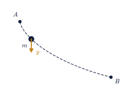
Fig. 156 The brachistochrone problem: a bead slides without friction from rest at \(A\) to the lower point \(B\) under gravity \(g\), along a curve \(y(x)\) to be chosen. Energy conservation fixes the speed \(v=\sqrt{2g(y_0-y)}\) at each height, so the descent time is the functional of Eq. 168; the dashed curve is one candidate path.#
Solution — Exercise 1#
straight-line descent time: numeric 1.188923 s, closed form 1.189043 s
Validation 1#
✓ straight-line descent time matches the closed form [got 1.18892 vs expected 1.18904 (rtol=0.001, atol=1e-09)]
True
Exercise 2 — The variational derivation of the cycloid#
Apply the Euler–Lagrange machinery to Eq. 168. Because the integrand \(F=\sqrt{1+y'^2}/\sqrt{-2gy}\) carries no explicit \(x\), the Beltrami identity Eq. 170 applies. Computing \(F-y'\,\partial F/\partial y'\) and simplifying gives the compact first integral
a separable first-order ODE. Its solution, parametrised by the rolling angle \(\varphi\), is exactly the cycloid Eq. 171. Rather than grind the separation by hand, we verify the cycloid against the first integral symbolically with SymPy: the same hand-vs-symbolic discipline as §2.1.
Form \(y'(\varphi)=\dot y/\dot x\) for the cycloid (
sympy.diff).Show \(y(1+y'^2)\) simplifies to the constant \(-2a\) (
sympy.simplify), i.e. the cycloid satisfies the brachistochrone first integral derived from Eq. 170.
y'(φ) = sin(varphi)/(cos(varphi) - 1)
y·(1 + y'²) = -2*a
Validation 2#
✓ the cycloid solves the brachistochrone first integral y(1+y'²)=const [y(1+y'²) = -2*a]
True
Exercise 3 — The cycloid beats the competition#
The variational argument says the cycloid is stationary; here we confirm it is the minimum by racing it, as a descent time, against two honest rivals between the same endpoints: the straight line and a curve that bows below the chord (a tuned sag). One caution sets up the computation: \(v=\sqrt{-2gy}\) is real only while \(y\le y_0=0\), so any rival must stay at or below the start height: a curve that rises above \(A\) would make the speed imaginary. Our sag \(y(x)=-\tfrac{2}{\pi}x - d\sin x\) (with \(d>0\)) dips below the chord yet never rises above \(A\).
Sampling is not the only way to time a descent. When the curve is known explicitly as \(y(x)\), Eq. 168 is a one-dimensional quadrature — except that the integrand blows up like \(1/\sqrt{x}\) at the start, where the bead is still at rest. The singularity is integrable, and the substitution \(x=u^2\) (with \(dx = 2u\,du\)) removes it outright, leaving a finite integrand a general quadrature routine can handle. The cycloid’s own time needs no quadrature at all: it is \(\pi\sqrt{a/g}\) in closed form (Exercise 4).
Write
descent_time_func(y_func, yp_func, x_end, g=G, y0=0.0), the descent time for an explicit curve: apply the substitution above to Eq. 168 and integrate withscipy.integrate.quadfrom \(u=0\) to \(u=\sqrt{x_\text{end}}\). Write this one yourself — the implementation is the lesson.Compute the descent times along the cycloid (closed form), the straight line, and the sag, and show the cycloid is fastest (Fig. 157).
cycloid : 1.0030 s (= π√(a/g))
line : 1.1890 s
sag : 1.0459 s
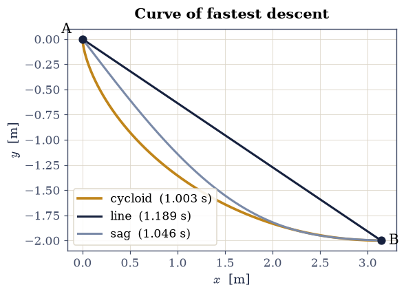
Fig. 157 Three frictionless descent paths between the same endpoints \(A=(0,0)\) and \(B=(\pi a,-2a)\), with their descent times: the cycloid (amber) is fastest at \(\pi\sqrt{a/g}\), beating both the straight line (dark) and a curve bowed below the chord (grey). The cycloid’s head start — plunging steeply at first to build speed — more than makes up for its longer arc.#
Validation 3#
✓ the cycloid is the curve of fastest descent [cycloid 1.003 < line 1.189, sag 1.046]
True
Exercise 4 — Descent time along the cycloid, in closed form#
On the cycloid the descent time has a clean closed form. Measuring arclength \(s\) from the low point, one finds \(s=4a\cos(\varphi/2)\) and that the height above the bottom is \(s^2/(8a)\), so a bead on the cycloid obeys \(\ddot s = -\tfrac{g}{4a}\,s\), simple harmonic motion with \(\omega=\tfrac12\sqrt{g/a}\). A bead released from the cusp (\(\varphi=0\)) reaches the bottom in a quarter period, \(T=\pi\sqrt{a/g}\): the result Eq. 172 (and reaching angle \(\varphi\) takes \(\varphi\sqrt{a/g}\)). Rather than trust the quarter-period argument, we integrate the arclength dynamics and let the solver report the arrival time itself.
Write
descent_time_ode(phi0, a=A_RAD, g=G): release the bead from rest at arclength \(s_0=4a\cos(\varphi_0/2)\), integrate \(\ddot s=-\omega^2 s\) withscipy.integrate.solve_ivpat tight tolerances, and stop the solve on a terminal, downward-crossing event at \(s=0\) — the arrival at the bottom — returning that event time. Write this one yourself — the implementation is the lesson.Release from the cusp (\(\varphi_0=0\)) and confirm the descent-to-bottom time equals \(\pi\sqrt{a/g}\).
cycloid descent-to-bottom time: numeric 1.0030333404 s
closed form π√(a/g): 1.0030333404 s
Validation 4#
✓ cycloid descent-to-bottom time is π√(a/g) [got 1.00303 vs expected 1.00303 (rtol=1e-06, atol=1e-09)]
True
Exercise 5 — The tautochrone property#
Here is the headline. Because the arclength motion is simple harmonic with a frequency \(\omega=\tfrac12\sqrt{g/a}\) that does not depend on amplitude, the time to reach the bottom is a quarter period whatever the release point: the tautochrone property Eq. 172. Release one bead from just above the bottom and another from the cusp: they arrive together.
With the
descent_time_odeyou wrote in Exercise 4, compute the descent-to-bottom time for several release angles \(\varphi_0\) spread over the arch, and confirm they are all equal to \(\pi\sqrt{a/g}\).
φ₀ = 0.0° → descent time = 1.0030333404 s
φ₀ = 30.0° → descent time = 1.0030333404 s
φ₀ = 60.0° → descent time = 1.0030333404 s
φ₀ = 90.0° → descent time = 1.0030333404 s
φ₀ = 120.0° → descent time = 1.0030333404 s
φ₀ = 150.0° → descent time = 1.0030333404 s
Validation 5#
✓ every start point reaches the bottom in the same time (tautochrone) [max|Δ| = 2.91989e-13 (rtol=1e-06, atol=1e-09)]
True
Exercise 6 — Synchronized beads (worked animation)#
Motion is the whole point of the tautochrone, so this is genuinely an animation. Place several beads at different heights on the same cycloid, release them all from rest at the same instant, and watch them slide down: they reach the lowest point in unison despite the different starts. The arclength SHM gives each bead’s position exactly: \(\varphi(t)=2\arccos\!\big(\cos(\varphi_0/2)\cos\omega t\big)\). The validation checks the physics of the animated data (that the arrival times agree), not the drawing.
Fig. 158 Animation of beads released from rest at different heights on a single cycloid (amber track): all reach the lowest point simultaneously — the tautochrone property, because motion along the cycloid is simple harmonic in arclength with an amplitude-independent frequency \(\omega=\tfrac12\sqrt{g/a}\).#
Validation 6#
Integrating each bead’s dynamics independently with the descent_time_ode you
wrote in Exercise 4, all arrival times must agree.
✓ all beads arrive at the bottom simultaneously [max|Δ| = 2.34923e-13 (rtol=0.001, atol=1e-09)]
True
Exercise 7 — The brachistochrone race (student animation)#
Now a race, where motion is again the point: release three beads at the same instant from \(A\), each constrained to a different track (cycloid, straight line, sag) all ending at \(B\). The cycloid bead wins, even though its path is longer, because it plunges early to build speed. Here you build the animation.
The dynamics along an arbitrary track follow from \(\ddot s = -g\,\frac{dy}{ds}\), the tangential component of gravity, with \(s\) the arclength along the track — the same equation the cycloid turned into simple harmonic motion in Exercise 4, but now with a slope \(dy/ds\) that varies from track to track. The cycloid bead needs no integration at all: its exact SHM solution already places it at any time.
Write
race_curve(xcv, ycv, t_frames, g=G), the bead motion along an arbitrary sampled track: build the cumulative arclength \(s\) along the samples, interpolate \(dy/ds\) and the coordinates \(x(s), y(s)\) against it, integrate \(\ddot s = -g\,dy/ds\) from rest withscipy.integrate.solve_ivp(dense output, plus a terminal event at the track’s end), and return the bead’s positions att_framestogether with its arrival time. Write this one yourself — the implementation is the lesson.Obtain each bead’s position over time:
race_curvefor the line and the sag, the closed-form SHMbead_xyof Exercise 6 for the cycloid, whose arrival time comes from your Exercise 4descent_time_ode.Animate the three beads racing, then
plt.close(fig)and end withecp.animate.show(anim).Confirm the cycloid bead arrives first by comparing the three arrival times.
A ✗ points at the descent integration or arrival times, not the animation.
arrivals — cycloid 1.003 s, line 1.189 s, sag 1.046 s
Fig. 159 Animation of three beads released together from \(A\) down a cycloid (amber), a straight line (dark), and a sag curve (grey) to the same point \(B\): the cycloid bead reaches \(B\) first despite travelling the longest arc, because it descends steeply at the outset to gain speed early — the brachistochrone advantage.#
Validation 7#
✓ the cycloid bead wins the race [cycloid 1.003 s < line 1.189 s, sag 1.046 s]
True
Notebook summary#
The descent-time functional \(T[y]=\int\sqrt{(1+y'^2)/(-2gy)}\,dx\) and its variational minimisation to the cycloid, confirmed to beat the straight line and a curve bowed below the chord.
The closed-form descent time along the cycloid; the tautochrone property (equal descent time from any starting height), shown with synchronized beads; and a brachistochrone race.
Outlook#
Snell’s law / Fermat’s principle. Johann Bernoulli’s own 1696 solution recast the bead as a light ray refracting through ever-faster media: the brachistochrone as an optics problem, and a first glimpse of the deep tie between least-time and least-action.
Huygens’ isochronous pendulum. A pendulum forced onto a cycloidal path is exactly isochronous: its period is independent of amplitude, unlike the circular pendulum of §1.2 whose period grows with swing. The tautochrone is why.
Constrained variation. Isoperimetric problems (the catenary, the hanging chain from the “going further” of §1.7, and the shape of a soap film) add a constraint via a Lagrange multiplier.
Geodesics as variational problems (the shortest path on a curved surface) point forward to general relativity.