3.4 Laplace’s and Poisson’s Equations

Elementary Computational Physics

Volume III — Classical Electrodynamics Notebook 3.4

The boundary-value problem and how to solve it: relaxation methods (Jacobi, Gauss–Seidel, SOR) and their convergence, the sparse linear-system view, sources via Poisson, and the method of images. The computational heart of the volume — long, and worth it.

Level · advanced   •   Est. · 150–200 min

Raymond Amador v1.4.0  ·  2026-07-31  ·  CC BY 4.0 (text) / MIT (code)

Notebook overview

A frank word before we start: this is a long notebook, and deliberately so. The boundary-value problem and the solvers we build for it are the computational core that the rest of this volume, and a surprising amount of the rest of physics, rests on. We would rather develop it once, carefully and whole, than scatter it thinly. It earns its length, and it is, we think, the most rewarding chapter in the volume.

Here the question of electrostatics turns inside out. §3.1–§3.3 worked in one direction: given the charges, sum or integrate for the field. But most real problems hand us the opposite. We are told the boundaries (the potentials on conductors, the voltages on walls) and asked for the field that fills the space between them. That is the boundary-value problem, and summing Coulomb’s law cannot touch it: we do not know where the charges (induced on the conductors) even are. We need genuinely new machinery, and we build it.

The notebook runs in four movements. I — discretization and relaxation: the five-point Laplacian, and solving Laplace’s equation by iterated neighbour-averaging (Jacobi), watched as it happens. II — convergence and the linear-system view: why Gauss–Seidel beats Jacobi, how successive over-relaxation (SOR) beats both at the right \(\omega\), and the recognition that the whole thing is one big sparse linear system that a direct solver can crack too. III — sources: Poisson’s equation, fields with no closed form. IV — the method of images: the elegant trick that turns special geometries into a few fictitious charges, cross-checked against relaxation. We close on the realisation that \(\nabla^2\varphi = \text{source}\) is the equation of equilibrium everywhere in physics, not just here.

Everything is in SI units (\(\varepsilon_0 = 8.854\times10^{-12}\,\)F/m). We work in 2-D throughout, where the fields and the convergence are easy to see and to animate; the methods generalise to 3-D essentially unchanged (only the pictures get harder), which we note where it matters.

How to read the checks. Each exercise ends with a validate call against an independent fact: a discrete Laplacian that vanishes, a relaxed field that matches an analytic series, a direct solve that matches relaxation, an image construction that zeroes the potential on a conductor. A ✓ is strong evidence; a ✗ is a prompt to locate the discrepancy, not a verdict.

Scope. A working review, not a numerical-analysis course. See Nolting, Theoretical Physics 3 [Nol16]; Griffiths, Introduction to Electrodynamics [Gri17] (ch. 3); Press et al., Numerical Recipes [PTVF07] (ch. 20, relaxation/PDEs); and Trefethen & Bau [TB97] for the iterative-methods/spectral-radius view.

Theory in brief

Laplace, Poisson, and uniqueness

Combining \(\mathbf E = -\nabla\varphi\) (§3.2) with Gauss’s law \(\nabla\cdot\mathbf E = \rho/\varepsilon_0\) (§3.3) gives the equation the potential obeys,

(205)\[\nabla^2\varphi = -\frac{\rho}{\varepsilon_0}\quad\text{(Poisson)}, \qquad \nabla^2\varphi = 0\quad\text{(Laplace, where }\rho=0\text{)} .\]

The uniqueness theorem is what makes this useful: in a region where \(\varphi\) is fixed on the entire boundary (Dirichlet conditions), Poisson’s equation has exactly one solution. So however we find a solution that obeys the equation and matches the boundary, it is guaranteed to be the solution. That licence (any valid solution is the solution) is what lets a numerical guess-and-relax procedure be trusted.

The mean-value property

A function with \(\nabla^2\varphi=0\) is called harmonic, and harmonic functions have a remarkable property (Griffiths [Gri17], ch. 3, gives the short proof): the value at any point equals the average of the values on any sphere (in 2-D, circle) centred there,

(206)\[\varphi(\mathbf r) = \big\langle \varphi \big\rangle_{\text{sphere about }\mathbf r} .\]

An immediate corollary: a harmonic function can have no local maximum or minimum in the interior (a peak would exceed its own surrounding average). The extremes live on the boundary. This is Earnshaw’s theorem again (callback to §3.2: no stable electrostatic trap), and it is the conceptual seed of everything below.

Discretizing the Laplacian

On a grid of spacing \(h\), a Taylor expansion gives the five-point stencil,

(207)\[\nabla^2\varphi \approx \frac{\varphi_{i+1,j}+\varphi_{i-1,j}+\varphi_{i,j+1}+\varphi_{i,j-1}-4\varphi_{i,j}} {h^2} .\]

Setting it to zero rearranges to \(\varphi_{i,j} = \tfrac14(\varphi_{i+1,j}+ \varphi_{i-1,j}+\varphi_{i,j+1}+\varphi_{i,j-1})\): each point is the average of its four neighbours, the mean-value property in discrete form.

Relaxation as iterated averaging

That rearrangement is also an algorithm: sweep the grid, replace each interior point by its neighbour-average (plus a source term for Poisson), and repeat until nothing changes. The boundary values, held fixed, diffuse inward to the harmonic solution. Three schemes differ only in when updated values are used:

• Jacobi Eq. 208: update every point from the values of the previous sweep.

  (208)\[\varphi^{k+1}_{i,j} = \tfrac14\big(\varphi^{k}_{i+1,j}+\varphi^{k}_{i-1,j} +\varphi^{k}_{i,j+1}+\varphi^{k}_{i,j-1}\big) + \tfrac{h^2}{4}\,\frac{\rho_{i,j}}{\varepsilon_0}.\]

• Gauss–Seidel Eq. 209: use neighbours already updated this sweep. Roughly twice as fast, and it needs no second copy of the grid.

  (209)\[\varphi^{k+1}_{i,j} = \tfrac14\big(\varphi^{k}_{i+1,j}+\varphi^{k+1}_{i-1,j} +\varphi^{k}_{i,j+1}+\varphi^{k+1}_{i,j-1}\big) + \tfrac{h^2}{4}\,\frac{\rho_{i,j}}{\varepsilon_0}.\]

• SOR (successive over-relaxation) Eq. 210: take the Gauss–Seidel step and overshoot it by a factor \(\omega\in(1,2)\). At the right \(\omega\) this is dramatically faster.

  (210)\[\varphi^{k+1}_{i,j} = (1-\omega)\,\varphi^{k}_{i,j} + \omega\,\varphi^{\text{GS}}_{i,j}.\]

Convergence: splittings and the spectral radius

Every such scheme is a linear iteration \(\boldsymbol\varphi_{k+1} = M\boldsymbol \varphi_k + \mathbf c\), and the error after each sweep is multiplied by the matrix \(M\). The error therefore shrinks by the spectral radius \(\rho(M)\) (the largest eigenvalue magnitude, callback to §0.5) per sweep,

(211)\[\|\mathbf e_{k}\| \sim \rho(M)^{\,k}\,\|\mathbf e_0\| .\]

Jacobi, Gauss–Seidel, and SOR are three different splittings of the same system matrix into “easy-to-invert plus remainder,” giving three different \(M\) and three different \(\rho(M)\), hence three convergence speeds. The smaller \(\rho(M)\), the faster. For the model problem on an \(n\times n\) grid the optimal SOR parameter has a closed form (Press et al., Numerical Recipes [PTVF07], ch. 20, derives it from the Jacobi spectral radius),

(212)\[\omega_{\text{opt}} = \frac{2}{1+\sin(\pi/n)} ,\]

which pushes \(\rho(M)\) from \(\approx 1-O(h^2)\) (Jacobi/G–S, painfully close to 1) down to \(\approx 1-O(h)\), the difference between \(O(n^2)\) and \(O(n)\) sweeps.

The sparse linear-system view

The discrete equations Eq. 207 are nothing but a large linear system,

(213)\[A\,\boldsymbol\varphi = \mathbf b ,\]

with \(A\) the (very sparse) five-point-stencil matrix and \(\mathbf b\) holding the boundary values and sources. Relaxation is an iterative solver for it; a direct sparse solver (scipy.sparse.linalg.spsolve, an \(LU\) factorization, callback to §0.4) is the alternative. Direct is exact but memory-hungry; iterative is approximate but scales. Same system, two philosophies.

The method of images

For a few special boundary shapes the BVP can be solved exactly with a trick: replace the conductor by fictitious image charges placed so the boundary condition falls out by symmetry,

(214)\[\varphi(\mathbf r) = \frac{1}{4\pi\varepsilon_0}\sum_i \frac{q_i}{|\mathbf r-\mathbf r_i|}, \quad\text{real charges + images, chosen so }\varphi=0\text{ on the conductor.}\]

A charge \(q\) at height \(d\) above a grounded plane is, in the region above, equivalent to \(q\) plus an image \(-q\) at \(-d\). A charge \(q\) a distance \(d\) from the centre of a grounded sphere of radius \(a\) has the Kelvin image \(q' = -qa/d\) at \(b = a^2/d\). Images give exact answers for special shapes; relaxation handles any shape. Where both apply, they validate each other.

Setup

Setup holds the data and the instruments: the constants (\(\varepsilon_0\), the Coulomb constant \(k\), the plot colours), a builder for the model box’s grid and Dirichlet mask, and the analytic Fourier series that the box solutions are graded against. The notebook’s own machinery is not here — you build the five-point Laplacian in Exercise 1, Jacobi relaxation in Exercise 2, red–black SOR (Gauss–Seidel at \(\omega=1\)) in Exercise 4, the sparse direct solve in Exercise 6, and the image-charge potential in Exercise 9.

The Setup below holds this notebook’s data and instruments — nothing you are asked to build. It is collapsed so the building stays yours; expand it whenever you want the details.

Show code cell source

Hide code cell source

import numpy as np
import matplotlib.pyplot as plt
import scipy.sparse as sp
import scipy.sparse.linalg as spla
from matplotlib.animation import FuncAnimation

from ecp import draw, validate
from ecp.animate import show

from scipy.constants import epsilon_0 as EPS0  # vacuum permittivity, F/m

K = 1.0 / (4.0 * np.pi * EPS0)  # data: Coulomb constant ≈ 8.99e9 N·m²/C²
POS, NEG = "#c1121f", "#16213e"  # data: positive red, negative dark blue


# instrument: it lays out the model problem's geometry — a uniform grid on the unit
# square, three grounded edges and one live edge — which the notebook is handed rather
# than derives; the physics is in the solver that fills the interior.
def box_bc(N, V_top=1.0):
    """Boundary conditions for the unit-square box problem.

    Three grounded edges and a top edge held at ``V_top``, the canonical Dirichlet test case.

    Parameters
    ----------
    N : int
        Grid points per side.
    V_top : float, optional
        Potential on the top edge (default 1.0).

    Returns
    -------
    phi, fixed : numpy.ndarray
        The initialised field and the boolean mask of held nodes.
    """
    x = np.linspace(0.0, 1.0, N)
    y = np.linspace(0.0, 1.0, N)
    h = x[1] - x[0]
    phi0 = np.zeros((N, N))
    phi0[:, -1] = V_top  # top edge y=1
    fixed = np.zeros((N, N), bool)
    fixed[0, :] = fixed[-1, :] = fixed[:, 0] = fixed[:, -1] = True
    return x, y, phi0, fixed, h


# data: the exact separation-of-variables solution of the box problem, quoted from the
# theory above rather than derived here — the known truth the solvers are graded against.
def box_series(x, y, V_top=1.0, n_terms=80):
    """Analytic Fourier-series solution of the box problem.

    The exact separable solution (a sum of sinh/sin modes), the truth the
    relaxed field is checked against.

    Parameters
    ----------
    x, y : numpy.ndarray
        Coordinates in the unit square.
    V_top : float, optional
        Top-edge potential (default 1.0).
    n_terms : int, optional
        Number of series terms (default 80).

    Returns
    -------
    numpy.ndarray
        The analytic potential at ``(x, y)``.
    """
    X, Y = np.meshgrid(x, y, indexing="ij")
    phi = np.zeros_like(X)
    for n in range(1, 2 * n_terms, 2):  # odd n only
        a = n * np.pi
        ratio = (
            np.exp(a * (Y - 1.0))
            * (1.0 - np.exp(-2.0 * a * Y))
            / (1.0 - np.exp(-2.0 * a))
        )
        phi += (4.0 * V_top / (n * np.pi)) * np.sin(a * X) * ratio
    return phi

Movement I — Discretization and relaxation

Exercise 1 — Discretizing the Laplacian

Everything starts with the five-point stencil Eq. 207: it turns the differential operator \(\nabla^2\) into a weighted sum over a point and its four neighbours (Fig. 216). The deepest sanity check is that it sends harmonic functions to (nearly) zero, since those are exactly the functions \(\nabla^2\) annihilates. Two clean test functions are \(u = x^2 - y^2\) and \(u = xy\): both satisfy \(\nabla^2 u = 0\) exactly, and for these quadratics the central difference is exact, so the discrete Laplacian should return zero to round-off.

1. Write laplacian_5pt(phi, h), the five-point discrete Laplacian Eq. 207 on a uniform grid: the sum of the four neighbours minus four times the centre, divided by \(h^2\), evaluated on the interior with the edges left zero (a vectorised slice expression, no Python loop). Write this one yourself — the implementation is the lesson: every solver in this notebook is a rearrangement of this one operator.

2. Apply it on a \(41\times41\) grid over \([-1,1]^2\) to \(u=x^2-y^2\) and \(u=xy\), and confirm the discrete Laplacian is zero on the interior to machine precision, the discrete echo of \(\nabla^2 u = 0\).

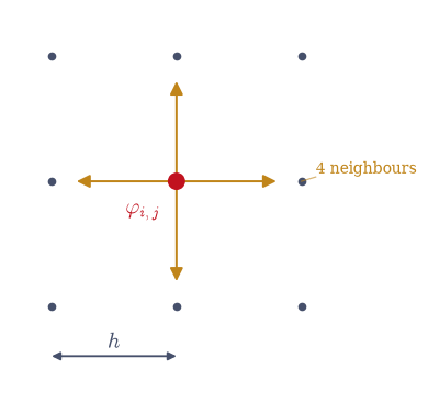
Fig. 216 The five-point stencil of Eq. eq-stencil: the discrete Laplacian at a grid node (red) is built from that node and its four nearest neighbours a step \(h\) away (amber). Laplace’s equation \(\nabla^2\varphi=0\) then says the centre value equals the average of the four neighbours, the mean-value property in discrete form.

max |discrete ∇²u| on the interior for u=x²−y² and u=xy: 3.55e-13

Validation 1

✓  the 5-point Laplacian of a harmonic function (x²−y², xy) is ≈ 0   [got 3.55271e-13 vs expected 0 (rtol=1e-06, atol=1e-10)]

True

Exercise 2 — Laplace by Jacobi relaxation

Now the central computation of the notebook. Take the unit square with three grounded edges and the top edge held at \(V_0 = 1\,\)V (Fig. 217). The interior potential is unknown; we find it by Jacobi relaxation Eq. 208, sweeping the grid and replacing every interior point by its neighbour-average until the largest change in a sweep drops below a tolerance. The boundary, held fixed, diffuses inward.

This box is one of the rare shapes with an analytic answer, a Fourier series \(\varphi(x,y) = \sum_{n\text{ odd}} \frac{4V_0}{n\pi}\sin(n\pi x)\frac{\sinh(n\pi y)}{\sinh(n\pi)}\), so we can grade relaxation against the truth. One honest caveat: the top corners are boundary discontinuities (the top edge is at \(V_0\), the sides at \(0\)), and there the discrete grid and the truncated series disagree by \(\sim V_0\), a Gibbs-type effect of the singular corner. We therefore compare on the interior, excluding the corner-adjacent nodes, and treat the corner mismatch as a lesson about boundary singularities rather than a failure.

On an \(N=40\) grid:

1. Write jacobi(phi, fixed, rhs, h, tol, max_iter, record), the Jacobi sweep Eq. 208: replace every interior node by the average of its four neighbours from the previous sweep plus \(\tfrac14 h^2\,\rho/\varepsilon_0\), write the result back only where the fixed mask is False, track the largest change of the sweep, and stop when it falls below tol (or at max_iter). Return the relaxed field, the sweep count, the history of changes, and — when record is non-zero — every record-th field, which Part 4 animates. Write this one yourself — the implementation is the lesson: this is the boundary-value solver the rest of the notebook is built on.

2. Relax from a zero initial guess to tolerance \(10^{-6}\) (max change per sweep).

3. Compare the result to the analytic Fourier series (box_series, given in Setup) on the interior nodes.

4. Then watch it happen: animate the field relaxing sweep by sweep (Fig. 218).

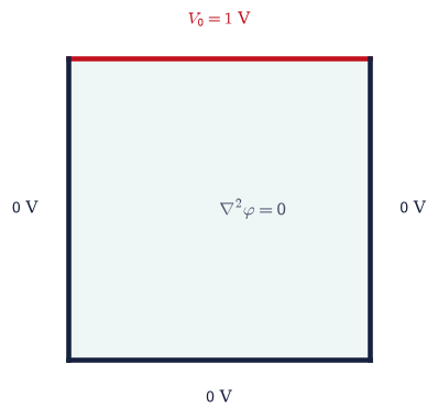
Fig. 217 The model boundary-value problem: the unit square with three grounded edges (\(0\,\)V) and the top edge held at \(V_0=1\,\)V. The interior potential is unknown and is found by relaxation; the only inputs are the values on the boundary (Dirichlet conditions), which uniqueness guarantees fix the interior.

Jacobi converged in 2212 sweeps (tol 1e-6)
max |Jacobi − analytic| on the interior (corners excluded): 2.36e-03

Validation 2

✓  Jacobi relaxation matches the analytic Fourier solution in the interior   [max|Δ| = 0.00236449 (rtol=1e-06, atol=0.005)]

True

The animation below shows the dynamics of convergence a still cannot: the top edge’s value spreading down into the square, fast at first then ever more slowly as the field settles onto the smooth harmonic solution.

Once Loop Reflect

Fig. 218 Animation of Jacobi relaxation on the box problem (\(N=40\), one frame per 10 sweeps): the potential, started at zero in the interior, relaxes as the top edge’s \(V_0\) diffuses inward. The change per sweep is large early and shrinks geometrically (Eq. eq-spectral-radius), so the picture moves fast then crawls, the visual signature of a spectral radius just below 1.

Exercise 3 — The mean-value property and no interior extremum

The converged field is harmonic, and harmonic functions obey the mean-value property Eq. 206: every interior value is the average of its neighbours. A corollary is no interior maximum or minimum (Earnshaw again, callback to §3.2): the hottest and coldest points sit on the boundary. Both are exact statements about the continuous solution and near-exact about our discrete one.

On the converged box solution of Exercise 2:

1. Confirm each interior point equals its four-neighbour average (a vectorised sliced-array average) to the relaxation tolerance.

2. Confirm the interior maximum and minimum (numpy.max/numpy.min) are strictly bracketed by the boundary’s (\(0\) and \(V_0\)).

max |φ − neighbour-average| on the interior: 9.94e-07
interior range [0.0007, 0.9483] strictly inside boundary [0, 1]: True

Validation 3

✓  the converged potential satisfies the mean-value property   [max|Δ| = 9.93822e-07 (rtol=1e-06, atol=1e-05)]
✓  no interior maximum or minimum: the extremes lie on the boundary (Earnshaw)

True

Movement II — Convergence and the linear-system view

Exercise 4 — Gauss–Seidel versus Jacobi

Jacobi throws away information: within a sweep it keeps using last sweep’s values even after better ones are available. Gauss–Seidel Eq. 209 uses each updated neighbour as soon as it is computed, which roughly halves the sweep count for the same accuracy. We compare them on the identical box problem to the identical tolerance.

Using fresh values sounds inherently sequential, but a red–black ordering rescues the vectorisation: colour the grid like a chessboard, and a point’s four neighbours are always of the other colour, so a whole colour can be updated at once from values of the opposite colour that are already current. Two half-sweeps make one Gauss–Seidel sweep. We write the routine once in its general form, with the over-relaxation factor \(\omega\) of Eq. 210 already in place — \(\omega=1\) is exactly Gauss–Seidel, and Exercise 5 turns the dial past it.

1. Write sor(phi, fixed, rhs, h, omega, tol, max_iter): split the free (non-fixed) nodes into the two chessboard colours; for each colour in turn form the Gauss–Seidel neighbour-average-plus-source, take the over-relaxed step \((1-\omega)\varphi + \omega\varphi^{\rm GS}\) Eq. 210, and apply it only on that colour’s nodes; track the largest change over the full sweep and stop below tol. Return the relaxed field, the sweep count, and the history of changes. Write this one yourself — the implementation is the lesson.

2. Relax the \(N=40\) box with the Jacobi routine you wrote in Exercise 2 and with Gauss–Seidel (sor at \(\omega=1\)) to tolerance \(10^{-6}\), and count the sweeps each needs (Fig. 219).

Jacobi:        2212 sweeps
Gauss–Seidel:  1214 sweeps   (1.82× fewer)

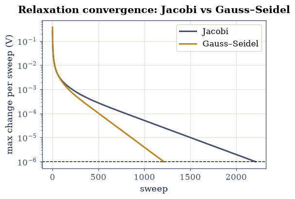
Fig. 219 Convergence of Jacobi versus Gauss–Seidel on the box problem (max change per sweep, log scale). Both decay geometrically (a straight line on this plot, Eq. eq-spectral-radius), but Gauss–Seidel’s slope is steeper: using already-updated neighbours shrinks the spectral radius, reaching the same tolerance in roughly half the sweeps.

Validation 4

✓  Gauss–Seidel converges in fewer iterations than Jacobi   [1214 vs 2212 sweeps]

True

Exercise 5 — SOR and the optimal \(\omega\)

The leap comes from over-relaxation Eq. 210: take the Gauss–Seidel correction and overshoot it by \(\omega\in(1,2)\). The reason it helps is the spectral-radius story Eq. 211: each scheme is a splitting of \(A\boldsymbol\varphi=\mathbf b\) into \(M\boldsymbol\varphi_k+\mathbf c\), and the error dies as \(\rho(M)^k\). For Jacobi and Gauss–Seidel \(\rho(M) = 1 - O(h^2)\) — agonizingly close to 1 on a fine grid, so \(O(n^2)\) sweeps. Over-relaxation tilts the splitting to minimize \(\rho(M)\), and at the optimum it drops to \(1 - O(h)\), i.e. \(O(n)\) sweeps. For the model problem the minimizer is known in closed form, \(\omega_{\text{opt}} = 2/(1+\sin(\pi/n))\) Eq. 212, and the iteration count has a sharp minimum there.

1. Sweep \(\omega\) across \((1, 2)\), running the sor routine you wrote in Exercise 4 to tolerance \(10^{-6}\) at each, and find the iteration-count minimum.

2. Compare the empirical best \(\omega\) to \(2/(1+\sin(\pi/(N-1)))\), and confirm SOR at the optimum is dramatically faster than Jacobi (Fig. 220).

empirical optimal ω = 1.860  (closed form 2/(1+sin(π/(N-1))) = 1.851)
SOR @ ω_opt: 90 sweeps   vs Jacobi 2212  (25× fewer)

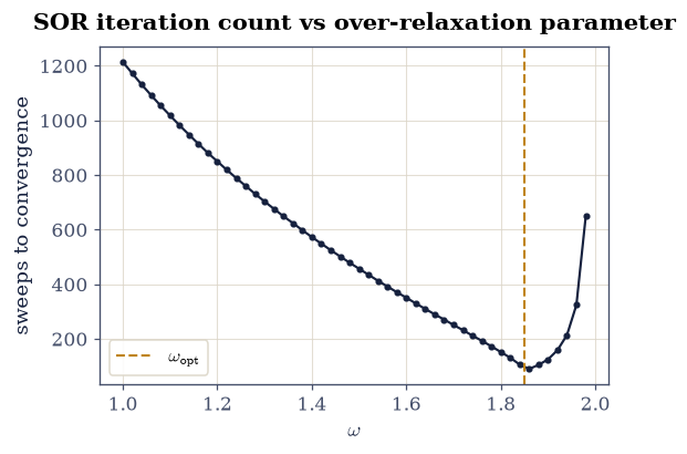
Fig. 220 Sweeps to convergence versus the over-relaxation parameter \(\omega\) for SOR on the box (\(N=40\), tolerance \(10^{-6}\)). The count plunges to a sharp minimum at \(\omega_{\mathrm{opt}}=2/(1+\sin(\pi/(N-1)))\) (dashed), then rises steeply toward \(\omega=2\). At the optimum SOR needs an order of magnitude fewer sweeps than Jacobi (Ex. 4) — the payoff of minimizing the iteration matrix’s spectral radius.

Validation 5

✓  the empirical optimal ω matches the closed form 2/(1+sin(π/(N-1)))   [got 1.86 vs expected 1.85105 (rtol=0.05, atol=1e-09)]
✓  SOR at the optimal ω is dramatically faster than Jacobi   [90 vs 2212 sweeps]

True

With your assistant

Relaxation solvers are a family, and your assistant knows more cousins than this notebook shows — ask it for one (red–black ordering, a multigrid V-cycle, whatever it offers) and run it on the boundary problem of Exercise 2. The gates are already built: the analytic solution of that exercise, and the mean-value property of Exercise 3, which any true harmonic solution must obey regardless of who wrote the iteration. The check is yours.

Exercise 6 — The sparse linear-system view (student)

Step back and look at what relaxation has been solving. The discrete equations Eq. 207 are a single linear system \(A\boldsymbol\varphi = \mathbf b\) Eq. 213: one row per interior node, \(-4\) on the diagonal and \(+1\) for each interior neighbour, with the known boundary values moved to the right-hand side \(\mathbf b\). The matrix is enormous but sparse (five non-zeros per row), so we store it with scipy.sparse and solve it directly with scipy.sparse.linalg.spsolve (a sparse \(LU\) factorization, callback to §0.4). The relaxation methods are simply iterative solvers of this very system, with speed set by the iteration matrix’s spectral radius (§0.5).

Assembling \(A\) is where the stencil becomes concrete: number the interior nodes, give each its own row with \(-4\) on the diagonal and \(+1\) in the column of every interior neighbour, and when a neighbour falls on the boundary its known value leaves the matrix and lands in \(\mathbf b\) instead. That last step is the whole content of a Dirichlet condition, seen algebraically.

1. Write solve_box_sparse(N, V_top): build the five-point-stencil matrix \(A\) for the \(N=40\) box as a scipy.sparse matrix, fold the Dirichlet boundary into \(\mathbf b\), solve \(A\boldsymbol\varphi=\mathbf b\) with scipy.sparse.linalg.spsolve, and reshape the interior solution back onto the grid. Write this one yourself — the implementation is the lesson: the matrix is the discretization, written out.

2. Confirm it matches the SOR relaxation (your Exercise 4 sor, at \(\omega_{\rm opt}\)) on the interior.

3. Weigh the trade-off: the direct solve is exact and needs no tolerance, but factorization fills memory; relaxation is approximate but scales to grids a direct solve could never hold.

sparse system size: 1444 × 1444, 5 non-zeros per interior row
max |direct spsolve − SOR relaxation| on the interior: 4.45e-08

Validation 6

✓  the direct sparse solve matches the relaxation solution   [max|Δ| = 4.45413e-08 (rtol=1e-06, atol=0.001)]

True

Movement III — Sources (Poisson)

Exercise 7 — Poisson with a source

Add charge and Laplace becomes Poisson Eq. 205, \(\nabla^2\varphi = -\rho/\varepsilon_0\). Relaxation barely changes: each averaging step simply gains the source term \(\tfrac14 h^2 \rho/\varepsilon_0\) Eq. 208. We place a smooth charge blob inside a grounded box (Fig. 221), relax for \(\varphi\), and recover the field \(\mathbf E = -\nabla\varphi\) by numerical gradient (§3.2).

In a grounded unit box (\(N=80\), all edges \(0\,\)V), place a Gaussian charge density \(\rho(x,y) = \rho_0\exp(-((x-\tfrac12)^2+(y-\tfrac12)^2)/2s^2)\) with \(s=0.06\) and a stated \(\rho_0\).

1. Relax with the sor routine you wrote in Exercise 4, at \(\omega_{\rm opt}\).

2. Verify the relaxed potential satisfies Poisson’s equation on the interior: its five-point Laplacian (the laplacian_5pt you wrote in Exercise 1) must equal \(-\rho/\varepsilon_0\).

3. Recover the field \(\mathbf E=-\nabla\varphi\) with numpy.gradient, plotting it over the potential (Fig. 222).

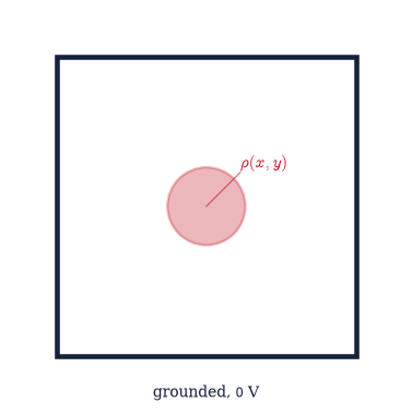
Fig. 221 The Poisson setup: a localized Gaussian charge blob (red) centred in a grounded unit box (all four edges at \(0\,\)V). The interior potential solves \(\nabla^2\varphi=-\rho/\varepsilon_0\); with no symmetry to exploit, relaxation is the tool.

Poisson relaxation: 228 SOR sweeps
max |∇²φ + ρ/ε₀| / max|ρ/ε₀| on the interior: 1.08e-06

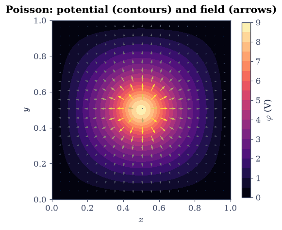
Fig. 222 The relaxed solution of Poisson’s equation for the Gaussian blob in a grounded box: filled contours of the potential \(\varphi\) with the field \(\mathbf E=-\nabla\varphi\) drawn by ecp.draw.field_quiver (arrow length and colour \(\propto|\mathbf E|\)). The field points outward from the positive charge and meets the grounded walls, where the induced surface charge terminates it.

Validation 7

✓  the relaxed potential satisfies Poisson's equation ∇²φ = −ρ/ε₀ in the interior   [got 1.08166e-06 vs expected 0 (rtol=1e-06, atol=0.02)]

True

Exercise 8 — A field with no closed form

Here is the payoff. Put two electrodes at different potentials inside a grounded box (Fig. 223) — a geometry with no series and no image solution. Relaxation does not care: it solves any shape. We mark the electrode nodes as fixed at their voltages and relax the charge-free region around them.

In a grounded unit box (\(N=80\)), hold a small left electrode at \(+1\,\)V and a small right electrode at \(-1\,\)V (stated rectangular patches).

1. Relax (your Exercise 4 sor, at \(\omega_{\rm opt}\)) for the field between them.

2. With no closed form to compare, check the solution against the physics it must obey: in the charge-free region it is harmonic, so the mean-value property Eq. 206 (a vectorised neighbour-average) must hold at every free interior node.

3. Recover the field \(\mathbf E=-\nabla\varphi\) with numpy.gradient (Fig. 224).

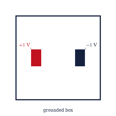
Fig. 223 An arbitrary geometry with no analytic solution: two electrodes, one at \(+1\,\)V (red) and one at \(-1\,\)V (blue), inside a grounded box. Series and image methods cannot touch this; relaxation solves it as readily as the box, which is the whole point of the numerical approach.

two-electrode relaxation: 195 SOR sweeps
max mean-value deviation on the charge-free interior: 4.40e-08

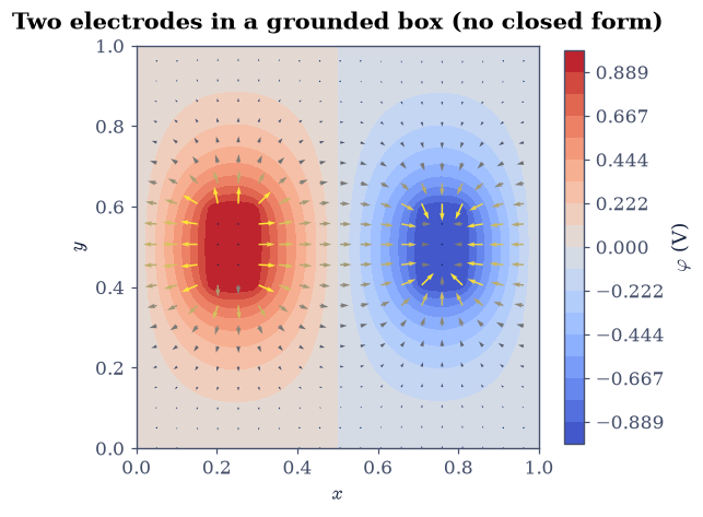
Fig. 224 The relaxed field of the two-electrode geometry: potential contours with \(\mathbf E=-\nabla\varphi\) (ecp.draw.field_quiver, arrows \(\propto|\mathbf E|\)). Field lines run from the \(+1\,\)V electrode to the \(-1\,\)V electrode and to the grounded walls. No closed form exists; the solution is trusted because it is harmonic (mean-value property) everywhere off the electrodes.

Validation 8

✓  the numerical solution is harmonic (mean-value property) in the charge-free region   [got 4.39949e-08 vs expected 0 (rtol=1e-06, atol=1e-05)]

True

Movement IV — The method of images

Exercise 9 — A charge above a grounded plane

For a few blessed geometries we can skip relaxation entirely. The classic is a charge above a grounded plane (Fig. 225): the grounded boundary at \(y=0\) can be reproduced exactly by deleting it and adding a fictitious image charge of opposite sign at the mirror position Eq. 214. Working in the 2-D slice (a line charge \(\lambda\) at height \(d\), image \(-\lambda\) at \(-d\)), the potential is a sum of two logarithms, and on the plane the two distances are equal, so \(\varphi=0\) falls out for free. Relaxation, given only the grounded boundary and the real charge, must reproduce it.

In 2-D the potential of a single line charge \(\lambda\) goes as \(-\lambda\ln r/(2\pi\varepsilon_0)\), so the image construction is a difference of two logarithms: one distance to the real charge, one to its mirror. Place a line charge at \((0.5, d)\) with \(d=0.3\) in the upper half of a box whose bottom edge is grounded.

1. Write phi_image_plane(X, Y), the potential of the real line charge at \((x_0, d)\) together with its image \(-\lambda\) at \((x_0, -d)\) Eq. 214, on coordinate grids X, Y. Write this one yourself — the implementation is the lesson: the whole method of images is the choice of that second term.

2. Verify it is zero on the grounded plane.

3. Relax the charge-free region with your Exercise 4 sor (bottom grounded; the far edges and a small contour around the charge set to the analytic potential, excising the singularity) and confirm relaxation fills it with the same field the image construction predicts.

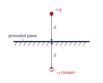
Fig. 225 The method of images for a charge \(+q\) at height \(d\) above a grounded plane (blue): in the region above the plane the field is identical to that of \(+q\) plus a fictitious image \(-q\) at depth \(-d\) (dashed, below the plane). The two are equidistant from every point of the plane, so their potentials cancel there and the grounded boundary condition \(\varphi=0\) is satisfied exactly.

max |φ_image| on the grounded plane: 0.00e+00
relaxation vs image on the charge-free region: 3.04e-03 (402 sweeps)

/tmp/ipykernel_3235/3320728198.py:59: RuntimeWarning: invalid value encountered in subtract
  img_vs_relax = float(np.max(np.abs((phi_relax_i - phi_img)[free_i])))

Validation 9

✓  the image construction gives zero potential on the grounded plane   [got 0 vs expected 0 (rtol=1e-06, atol=1e-12)]
✓  relaxation reproduces the image-charge solution in the charge-free region   [max|Δ| = 0.00303843 (rtol=1e-06, atol=0.005)]

True

Exercise 10 — Induced charge and the force on the real charge (student)

The image is fictitious, but the induced surface charge it stands in for is real. For the 3-D point charge \(q\) at height \(d\) above a grounded plane, the induced density is \(\sigma(r) = -qd/\big(2\pi(r^2+d^2)^{3/2}\big)\) at distance \(r\) from the foot of the charge. Two famous results follow: the induced charge totals exactly \(-q\), and the attractive force on \(q\) is exactly that of its image, \(F = kq^2/(2d)^2\) (the charge is pulled toward the plane as if a charge \(-q\) sat a distance \(2d\) away).

With \(q=1\,\)nC and \(d=0.05\,\)m:

1. Integrate \(\sigma(r)\) over the plane with numpy.trapezoid (in polar form, \(\int_0^\infty \sigma(r)\,2\pi r\,dr\)) and confirm it equals \(-q\).

2. Compute the force \(F=kq^2/(2d)^2\).

total induced surface charge ∫σ dA = -9.9900e-10 C  (−q = -1.0e-09 C)
force on the charge F = kq²/(2d)² = 8.9876e-07 N (toward the plane)

Validation 10

✓  the total induced surface charge equals −q   [got -9.98999e-10 vs expected -1e-09 (rtol=0.002, atol=1e-09)]
✓  the image force kq²/(2d)² equals the integrated pull of the real induced charge   [got 8.98755e-07 vs expected 8.98753e-07 (rtol=0.001, atol=1e-09)]

True

Exercise 11 — The grounded sphere

The cleverest image is Kelvin’s, for a grounded sphere of radius \(a\) (Fig. 226). A charge \(q\) a distance \(d>a\) from the centre is balanced, on the sphere, by a single image \(q' = -qa/d\) placed inside at \(b=a^2/d\) Eq. 214. The magic is that this one off-centre image makes the entire curved surface an equipotential at zero, which is far from obvious (Griffiths [Gri17], ch. 3, works the construction through).

With \(a=0.1\,\)m, \(d=0.25\,\)m, and \(q=1\,\)nC:

1. Construct the Kelvin image \(q'=-qa/d\) at \(b=a^2/d\).

2. Sample the sphere surface on a \((\theta,\varphi)\) grid (numpy.meshgrid) and evaluate the total potential (real charge + image) there, with point-to-charge distances from numpy.linalg.norm.

3. Confirm it is zero to round-off.

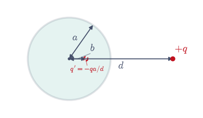
Fig. 226 Kelvin’s image for a grounded sphere of radius \(a\): a charge \(+q\) at distance \(d\) from the centre is matched by a single interior image \(q'=-qa/d\) at \(b=a^2/d\) (dashed). This one off-centre image makes the whole spherical surface an equipotential at zero potential.

Kelvin image: q' = -4.0000e-10 C at b = 0.0400 m
max |φ| on the sphere surface, relative to kq/a: 4.14e-16

Validation 11

✓  the Kelvin image q′=−qa/d at b=a²/d makes the sphere surface an equipotential at zero   [got 4.1359e-16 vs expected 0 (rtol=1e-06, atol=1e-12)]

True

Exercise 12 — The Laplacian everywhere

A closing widening of the lens. Nothing in Movements I–III was specific to electrostatics. The equation \(\nabla^2\varphi = \text{source}\), solved subject to boundary conditions, is the equation of equilibrium across physics: it is steady-state heat conduction (with \(\varphi\) the temperature and the source a heat input), incompressible irrotational flow (with \(\varphi\) the velocity potential), the shape of a stretched soap film (the minimal surface), and the smoothness of the quantum ground state. The relaxation solver we built does not know or care which it is.

Read the box problem of Exercise 2 as steady-state heat instead: a square plate with three edges held at \(0^\circ\) and the top edge at \(1^\circ\), at thermal equilibrium. The governing equation is the same Laplace equation, so the same relaxation must give the same field.

1. Solve the “heat” problem with your Exercise 4 sor at \(\omega_{\rm opt}\) and confirm it reproduces the electrostatic solution of Exercise 6 exactly — same math, relabelled.

max |steady-state heat − electrostatic potential| on the interior: 0.00e+00

Validation 12

✓  the same relaxation solves the steady-state heat problem (same equation, relabelled)   [max|Δ| = 0 (rtol=1e-06, atol=1e-06)]

True

The Laplacian is the operator of equilibrium. Wherever a system settles into the smoothest field consistent with what is fixed on its boundary — a potential between conductors, a temperature across a plate, a flow around an obstacle — the same \(\nabla^2\varphi=\text{source}\) governs it, and the same relaxation and sparse-solver machinery built here will crack it. That reach is why this notebook earned its length.

Notebook summary

• Laplace’s and Poisson’s equations solved by relaxation: Jacobi and Gauss–Seidel iteration to a fixed boundary-value problem, with the animation showing \(V\) diffusing inward and the change per sweep shrinking geometrically (spectral radius just below 1).

• The mean-value property and the no-interior-extremum theorem (Earnshaw) confirmed on the converged field; SOR accelerating convergence; and Poisson’s equation with a source.

• The sparse linear-system view: the five-point matrix solved directly with scipy.sparse.linalg.spsolve and matching relaxation; a two-electrode field with no closed form trusted through the mean-value property; and the method of images (grounded plane, induced charge totalling \(-q\), Kelvin’s sphere) cross-validated against relaxation — closing with the Laplacian as the equation of equilibrium everywhere (the same solve, relabelled as steady-state heat).

Outlook

• Multigrid methods. Relaxation kills short-wavelength error fast but long-wavelength error agonizingly slowly. Multigrid solves the problem on a hierarchy of grids, curing every wavelength on the scale where it is local; it beats even optimal SOR and is the modern fast Poisson solver.

• Conjugate gradient. The sparse system \(A\boldsymbol\varphi=\mathbf b\) is symmetric positive-definite, so conjugate gradient solves it in far fewer steps than relaxation, especially with a preconditioner. The Outlook of §0.4 names the method for the same reason; neither notebook builds it, so this is an outward horizon rather than a forward link to machinery the course delivers.

• Other boundary conditions. Neumann (fixed normal derivative, e.g. an insulated wall) and mixed conditions need only a tweak to the stencil at the boundary; the finite-element method handles complicated geometries with unstructured meshes.

• Three dimensions. Everything here generalizes by adding a third index and two more neighbours to the stencil; only the visualization gets harder.

• More images. Two parallel grounded planes need an infinite train of images; a point charge and a dielectric interface, a pair of fractional images. The method is a small art of its own.

References

[Gri17] (1,2,3)

David J. Griffiths. Introduction to Electrodynamics. Cambridge University Press, 4 edition, 2017.

[Nol16]

Wolfgang Nolting. Theoretical Physics 3: Electrodynamics. Springer, 2016.

[PTVF07] (1,2)

William H. Press, Saul A. Teukolsky, William T. Vetterling, and Brian P. Flannery. Numerical Recipes: The Art of Scientific Computing. Cambridge University Press, 3 edition, 2007.

[TB97]

Lloyd N. Trefethen and David Bau. Numerical Linear Algebra. Society for Industrial and Applied Mathematics (SIAM), 1997.

Take this notebook with you

Use the download button (↓) in the toolbar above to save this notebook and run it yourself. The published notebooks ship without worked solutions; if you would like the reference solutions — to teach from or to check your own work — get in touch: hello@ramador.me.