


5.2 Probability: Distributions, Expectation, and the Born Rule#
Notebook overview#
§5.1 taught us to count configurations. This one turns those counts into probabilities, the language physics actually speaks, and it carries a payload worth announcing up front. The two quantities we build here — the expectation \(\langle A\rangle\) and the variance, whose square root is the standard deviation — are not merely the average and the spread of a distribution. They are, letter for letter, the objects quantum mechanics calls the expectation value of an observable and its uncertainty \(\Delta A\). The Heisenberg uncertainty principle is a statement about variances. So we define these things in their physics form from the first line, and when observables become operators in Volume VI, the definitions will transfer without a single change.
We build patiently. First the bridge from counting: for equally likely outcomes a probability is just favourable microstates over total microstates, and the requirement that all probabilities sum to one is — we flag it immediately — the very normalization \(\langle\psi| \psi\rangle=1\) that the Born rule will demand of a quantum state. Then conditional probability and Bayes’ theorem, treated carefully as the disciplined updating of a sample space (not as the apparatus of statistical inference, which belongs to a different subject). Then the distributions physical systems actually realize: the binomial of a two-state paramagnet, the multinomial of an energy partition, the geometric waiting time, and — in full — the Poisson law of rare events that governs radioactive decay, photon counting, and shot noise. We show the binomial becomes Poisson in the rare-event limit, and we close on the expectation and variance themselves, the Born-rule heart of the notebook.
Throughout we lean on Monte Carlo — estimating probabilities by simulation with
numpy.random.default_rng — both as confirmation and as a preview, since Monte Carlo is the
engine that drives this volume’s physics from §5.4 onward. We verify our hand-built
distributions against scipy.stats (used only as an independent check, never as a
substitute for building them ourselves), and we reuse the ecp.combinatorics schematics and
distribution-bar plots from §5.1.
How to read the checks. Each exercise closes with a
validatecall against an independent fact: probabilities summing to one; \(P(\text{sum}=8)=5/36\); Bayes reversing the conditioning; the hand-built binomial and Poisson matchingscipy.stats; the Poisson signature \(\langle k\rangle=\mathrm{Var}=\lambda\); the die’s \(\langle A\rangle=3.5\) and \(\mathrm{Var}=35/12\); variances of independent variables adding. A ✓ is strong evidence; a ✗ is a prompt to locate the discrepancy, not a verdict.Scope. Probability as the language of microstate statistics; the large-\(N\) limit (Stirling, the CLT, the sharpness of macrostates) is §5.3, and the physics begins at §5.4. See Feller, An Introduction to Probability Theory; Schroeder, Thermal Physics; and Volume VI (the Born rule, where \(\langle A\rangle\) and \(\Delta A\) return as operators).
Theory in brief#
From counts to probability#
For equally likely outcomes, a probability is a ratio of counts,
A sample space lists the mutually exclusive outcomes; their probabilities are non-negative and sum to one. Flag this normalization now: it is exactly the quantum normalization \(\langle\psi|\psi\rangle=1\). Probabilities are the structure the Born rule will make physical.
Conditional probability and Bayes’ theorem#
Conditioning on an event \(B\) restricts the sample space to \(B\),
Bayes’ theorem (the middle equation) reverses the conditioning; here it is pure conditional probability — the updating of a sample space — not statistical inference. Independence, the last equation, is the physical statement that separate subsystems multiply their probabilities, which becomes product states and additive entropy.
The physical distributions#
Four distributions carry most of statistical physics,
The binomial counts successes in \(n\) independent two-outcome trials (a two-state system), with \(\langle k\rangle=np\) and \(\mathrm{Var}=np(1-p)\). The multinomial generalises it to several outcomes (an energy partition). The geometric is the waiting time to the first success, mean \(1/p\). The Poisson is the limit of the binomial for many rare events (\(n\to\infty\), \(p\to0\), \(np=\lambda\) fixed); its signature is \(\langle k\rangle=\mathrm{Var}= \lambda\), and it governs radioactive decay, photon arrivals, and shot noise.
Expectation and variance — the Born-rule heart#
The two summary numbers are
Read them as physics. \(\langle A\rangle\) is the expectation value of an observable, and \(\Delta A=\sqrt{\mathrm{Var}(A)}\) is its uncertainty — the very \(\Delta x\), \(\Delta p\) of the Heisenberg relation. Expectation is linear, and for independent variables variances add, \(\mathrm{Var}(X+Y)=\mathrm{Var}(X)+\mathrm{Var}(Y)\).
Monte Carlo: probability by simulation#
A probability or expectation can be estimated by sampling,
the estimate converging to the truth as \(1/\sqrt N\) — the seed of the Monte Carlo methods that become this volume’s spine from §5.4.
Setup#
Data and instruments only: the series palette and the §5.1 drawing
helpers from ecp.combinatorics, which render the distribution bars. This notebook’s own
constructs are not here. You write the binomial pmf and the two Born-rule quantities —
binomial_pmf, expectation and variance — in Exercise 4, and the Poisson pmf
poisson_pmf in Exercise 6; everything downstream, including the rare-event limit and the
fair-die uncertainty, runs on them. Each Monte Carlo below seeds its own
numpy.random.default_rng where it is used, so every sampled number on this page is
reproducible.
The Setup below holds this notebook’s data and instruments — nothing you are asked to build. It is collapsed so the building stays yours; expand it whenever you want the details.
Exercise 1 — From counts to probability (worked)#
Probability begins exactly where §5.1 left off. When outcomes are equally likely, the probability of an event is the fraction of microstates that realise it Eq. 387, so every count we computed last notebook is one division away from a probability. Take poker: the probability of being dealt a flush is its count over the total, \(5108/2598960\approx 0.0020\). Because every hand falls into exactly one category, the category probabilities must sum to one (Fig. 400) — and that requirement is not a bookkeeping nicety. It is the same condition the Born rule will impose on a quantum state, \(\langle\psi|\psi\rangle =1\): the probabilities of all the outcomes of a measurement must add to certainty.
The eight named hands are counted in §5.1; the ninth category, high card, is whatever is left over once they are subtracted from the total \(C(52,5)\). That remainder is the genuine test of the set, since only correct named counts leave the classic \(1{,}302{,}540\) behind.
Part a) Convert the §5.1 poker counts to probabilities: take the total
from math.comb, fix the high-card count as the remainder, divide each count by the total,
and tabulate the nine probabilities.
Part b) Confirm that the remainder lands on \(1{,}302{,}540\) and that the nine probabilities sum to \(1\) — the classical shadow of quantum normalization.
high card = C(52,5) − Σ(named) = 1,302,540  (classic value 1,302,540)
  P(straight flush  ) = 0.000015
  P(four of a kind  ) = 0.000240
  P(full house      ) = 0.001441
  P(flush           ) = 0.001965
  P(straight        ) = 0.003925
  P(three of a kind ) = 0.021128
  P(two pair        ) = 0.047539
  P(one pair        ) = 0.422569
  P(high card       ) = 0.501177

sum of all probabilities = 1.0000000000
Validation 1#
✓ the categories complete the deck (high card = 1,302,540) and the probabilities sum to 1
True
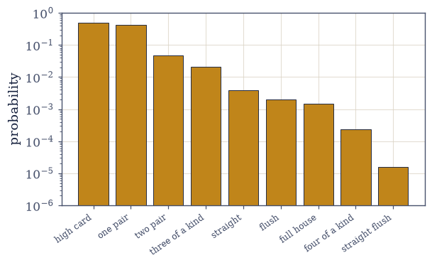
Fig. 400 The poker-hand probabilities (log scale), the §5.1 counts divided by \(C(52,5)\). They span four orders of magnitude — a high-card hand is over thirty thousand times more likely than a straight flush — yet they sum to exactly one (every hand is some category). That normalization, \(\sum_i p_i=1\), is the classical ancestor of the quantum condition \(\langle\psi|\psi\rangle=1\): the probabilities of all outcomes of a measurement must total certainty.#
Exercise 2 — Conditional probability (worked)#
A probability can change the moment we learn something. Conditional probability \(P(A\mid B)\) is the probability of \(A\) once we know \(B\) has happened, computed by restricting the sample space to \(B\) Eq. 388. Roll two dice: across all \(36\) equally likely outcomes, the sum is \(8\) in five of them (\(2{+}6,3{+}5,4{+}4,5{+}3,6{+}2\)), so \(P(\text{sum}=8)=5/36\). But if we are told the first die shows \(5\), the sample space shrinks to six outcomes, and only one of them (\(5{+}3\)) sums to \(8\), so \(P(\text{sum}=8\mid\text{first}=5)=1/6\) (Fig. 401). Learning the first die changed the probability.
The same enumeration settles independence. Each die is even with probability \(1/2\), so if the two are independent their probabilities must multiply, giving \(P(\text{both even})=P(\text{even})^2=1/4\). Independent subsystems multiplying their probabilities is what makes entropy additive (§5.4).
Part a) Enumerate the \(36\) outcomes with itertools.product and compute
\(P(\text{sum}=8)\), the conditional \(P(\text{sum}=8\mid\text{first}=5)\) by counting within the
restricted space, and \(P(\text{both even})\).
Part b) Confirm that \(P(\text{sum}=8)=5/36\) and that the two dice are independent, \(P(\text{both even})=1/4\).
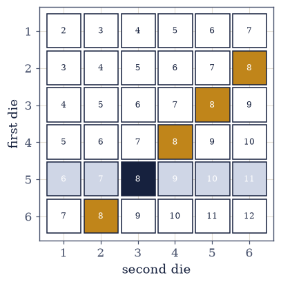
Fig. 401 Conditional probability restricts the sample space. Of the \(36\) equally likely rolls of two dice, five sum to \(8\), so \(P(\text{sum}=8)=5/36\). But learning the first die shows \(5\) (dark column) cuts the sample space to six outcomes, of which only \(5{+}3\) sums to \(8\) — so \(P(\text{sum}=8\mid\text{first}=5)=1/6\). Knowledge reshapes the space over which we count.#
P(sum=8)              = 0.1389  (= 5/36)
P(sum=8 | first=5)    = 0.1667  (= 1/6, the sample space shrank)
P(both even)          = 0.2500  vs P(even)² = 0.2500  (independent)
Validation 2#
✓  P(sum=8) = 5/36   [got 0.138889 vs expected 0.138889 (rtol=1e-09, atol=1e-09)]
✓  the two dice are independent: P(both even) = P(even)² = 1/4   [got 0.25 vs expected 0.25 (rtol=1e-09, atol=1e-09)]
True
Exercise 3 — Bayes’ theorem (worked)#
This one rewards going slowly. Bayes’ theorem reverses a conditional probability: it turns “the probability of the evidence given the cause” into “the probability of the cause given the evidence” Eq. 388. Here is a clean version. Two bags sit on a table. Bag \(A\) holds two red balls and one blue; bag \(B\) holds one red and two blue (Fig. 402). We pick a bag at random — each with probability \(\tfrac12\) — and draw one ball, which turns out red. What is the probability we drew from bag \(A\)?
Work it in pieces. The probability of red given \(A\) is \(P(R\mid A)=2/3\), and given \(B\) it is \(P(R\mid B)=1/3\). The overall probability of drawing red is the weighted average \(P(R)=P(R\mid A)P(A)+P(R\mid B)P(B)=\tfrac23\cdot\tfrac12+\tfrac13\cdot\tfrac12=\tfrac12\). Bayes then assembles these into the answer, \(P(A\mid R)=P(R\mid A)P(A)/P(R)=(\tfrac23\cdot\tfrac12)/\tfrac12=\tfrac23\). The red draw made bag \(A\) twice as likely as bag \(B\), exactly because \(A\) is twice as rich in red. This is conditional probability — the disciplined updating of a sample space once evidence arrives — not the separate machinery of statistical inference.
A direct enumeration is the independent check: run over every equally likely (bag, ball) outcome, weight each ball by the \(\tfrac12\) chance of its bag and the \(1/3\) chance of being drawn from it, and take the fraction of the red draws that came from \(A\). No theorem is used — only counting — so agreement between the two routes is real evidence.
Part a) Compute \(P(A\mid R)\) twice: once by Bayes’ theorem written out as explicit Python arithmetic, and once by that direct enumeration.
Part b) Confirm the two routes agree and that the posterior is \(2/3\).
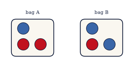
Fig. 402 A Bayes setup. Bag \(A\) holds two red and one blue ball; bag \(B\) holds one red and two blue. A bag is chosen at random and a red ball drawn. Because \(A\) is twice as rich in red, observing a red draw makes \(A\) twice as likely as \(B\) — Bayes’ theorem turns \(P(\text{red}\mid\text{bag})\) into \(P(\text{bag}\mid\text{red})=2/3\). It is the updating of a sample space once evidence arrives, nothing more.#
P(red)            = 0.5000
P(A | red) Bayes  = 0.6667  (= 2/3)
P(A | red) enum   = 0.6667  (agree)
Validation 3#
✓  Bayes' theorem reverses the conditioning correctly (matches direct enumeration)   [got 0.666667 vs expected 0.666667 (rtol=1e-12, atol=1e-09)]
✓  the red draw makes bag A twice as likely: P(A|red) = 2/3   [got 0.666667 vs expected 0.666667 (rtol=1e-09, atol=1e-09)]
True
Exercise 4 — The binomial distribution (worked)#
Our first full distribution, and the workhorse of statistical physics. Flip a coin \(n\) times, each flip independently heads with probability \(p\); the probability of getting exactly \(k\) heads is the binomial \(\binom{n}{k}p^k(1-p)^{n-k}\) Eq. 389 — the \(C(n,k)\) sequences of §5.1, each weighted by its probability. Its mean is \(\langle k\rangle=np\) and its variance \(\mathrm{Var}=np(1-p)\). This is exactly a two-state system: \(n\) spins each up or down, with \(k\) up. The distribution we plot here is, with spins for coins, the multiplicity distribution of a paramagnet (Fig. 403).
This is where the notebook’s tools get built, so it is worth knowing what each one is for.
The pmf itself is the distribution; the two summary numbers taken from it, the expectation
\(\langle A\rangle=\sum_i a_iP(a_i)\) and the variance \(\mathrm{Var}(A)=\langle A^2\rangle-
\langle A\rangle^2\) Eq. 390, are the Born-rule constructs the whole notebook is
built around — Exercise 8 returns to what they mean, and every distribution from here on is
measured with them. Note that math.comb and math.factorial take one integer at a time,
so a pmf evaluated on an array of counts must map them element by element and restore the
shape of the input. The animation flips coins with numpy.random.default_rng and watches the
histogram of head-counts build up toward the binomial curve (Fig. 403).
Part a) Write binomial_pmf(k, n, p), the probability \(\binom{n}{k}p^k(1-p)^{n-k}\)
Eq. 389 of exactly \(k\) successes in \(n\) trials, accepting an array of counts
k. Write this one yourself — the implementation is the lesson, and the rest of the
notebook runs on it.
Part b) Write expectation(values, probs) and variance(values, probs), the two
summaries Eq. 390 of an observable taking values with probabilities probs.
Write these yourself — the implementation is the lesson; these are the definitions
Volume VI will hand operators to.
Part c) For \(n=20\), \(p=0.4\), build the pmf over \(k=0,\dots,20\), compare it with
scipy.stats.binom.pmf (an independent referee, never the implementation), and take the mean
and variance from the pmf itself.
Part d) Confirm the hand-built pmf matches the library’s, and that \(\langle k\rangle=np\) and \(\mathrm{Var}=np(1-p)\).
binomial n=20, p=0.4:
  hand-built pmf matches scipy.stats.binom.pmf: True
  ⟨k⟩ = 8.0000  vs np   = 8.0
  Var = 4.8000  vs np(1−p) = 4.8
Validation 4#
✓  the hand-built binomial pmf matches the standard scipy.stats one   [max|Δ| = 3.88578e-16 (rtol=1e-09, atol=1e-09)]
✓  the binomial has ⟨k⟩=np and Var=np(1−p)   [max|Δ| = 1.68754e-14 (rtol=1e-09, atol=1e-09)]
True
Fig. 403 The binomial distribution emerging from coin flips (animated). Each trial flips \(n=20\) coins (\(p=0.4\) heads) with numpy.random.default_rng and records the number of heads; the bars show the running histogram as trials accumulate, converging onto the exact binomial pmf (dark markers). Mean \(\langle k\rangle=np=8\), variance \(np(1-p)=4.8\). Read spins for coins and this is the multiplicity distribution of a \(20\)-spin paramagnet.#
Exercise 5 — The multinomial and geometric distributions (worked)#
Two quick generalisations. The multinomial distribution counts the ways \(n\) trials split among several outcomes rather than two — the natural object when energy is partitioned among many levels. Roll six dice; the probability of seeing exactly one of each face is \(6!\,(1/6)^6\approx0.0154\): the \(6!\) orderings of “one of each” out of the \(6^6\) equally likely rolls. The geometric distribution is the waiting time to the first success in repeated trials, \(P(k)=(1-p)^{k-1}p\), with mean \(1/p\) — wait, on average, \(1/p\) trials for an event of probability \(p\).
Both claims are small enough to check exactly. The six-dice statement has only \(6^6=46{,}656\) outcomes, so it can be brute-forced; and the geometric mean is a convergent series whose terms fall off geometrically, so summing a few hundred of them is already indistinguishable from the closed form. The multinomial is worth the attention: it is the combinatorial form of partitioning energy among many levels (§5.4).
Part a) Compute the multinomial probability of one-of-each on six dice as \(6!\,(1/6)^6\)
with math.factorial, and check it against a brute-force enumeration of all \(6^6\) rolls with
itertools.product.
Part b) Compute the geometric mean \(\sum_k k(1-p)^{k-1}p\) for \(p=0.2\) as an explicit
numpy sum over \(k=1,\dots,499\).
Part c) Confirm the multinomial matches the enumeration and that the geometric mean equals \(1/p\).
multinomial P(one of each, six dice) = 6!·(1/6)⁶ = 0.01543
enumeration over all 6⁶ rolls          = 0.01543  (agree)
geometric mean (p=0.2) = Σ k(1−p)^(k−1)p = 5.0000  vs 1/p = 5.0
Validation 5#
✓ the multinomial matches brute-force enumeration and the geometric mean equals 1/p [max|Δ| = 1.77636e-15 (rtol=1e-06, atol=1e-09)]
True
Exercise 6 — The Poisson distribution (worked)#
The Poisson distribution is the law of rare events, and it deserves a full treatment because physics is full of it. When events happen independently at some average rate, the number \(k\) observed in a fixed interval follows \(P(k)=\lambda^k e^{-\lambda}/k!\) Eq. 389, where \(\lambda\) is the mean count. Its signature, which no other distribution shares, is that the mean equals the variance, \(\langle k\rangle=\mathrm{Var}= \lambda\) (Fig. 404). A detector clicking on average \(\lambda=3\) times a second, a sample emitting \(\lambda\) decays per minute, photons arriving at a sensor — all Poisson, and all forward pointers to the quantum counting of Volumes VI and VII.
Two ranges of \(k\) are needed below, and the distinction matters. The figure wants a short range, \(k=0,\dots,15\), because the bars beyond that are invisible; the moments, though, are sums over all \(k\), so truncating them early would bias \(\langle k\rangle\) and \(\mathrm{Var}\) downward. Taking \(k\) out to \(39\) puts the discarded tail below machine precision, and the moments are then exact for every purpose here.
Part a) Write poisson_pmf(k, lam), the probability \(\lambda^ke^{-\lambda}/k!\)
Eq. 389 of \(k\) events at mean count \(\lambda\), accepting an array of counts k
in the same element-by-element way as your Exercise 4 binomial_pmf. Write this one
yourself — the implementation is the lesson.
Part b) For \(\lambda=3\) (say, detector clicks per second) build the pmf on both ranges,
take \(\langle k\rangle\) and \(\mathrm{Var}\) from the long one with the expectation and
variance you wrote in Exercise 4, and draw \(200{,}000\) Monte Carlo counts with
rng.poisson as a further independent view.
Part c) Confirm the hand-built pmf matches scipy.stats.poisson.pmf and that
\(\langle k\rangle=\mathrm{Var}=\lambda\), the Poisson signature.
Poisson λ=3.0 (detector clicks per second):
  hand-built pmf matches scipy.stats.poisson.pmf: True
  ⟨k⟩ = 3.0000,  Var = 3.0000   (the Poisson signature: equal)
  Monte Carlo mean = 2.995, variance = 3.003
Validation 6#
✓  the hand-built Poisson pmf matches the standard scipy.stats one   [max|Δ| = 9.71445e-17 (rtol=1e-09, atol=1e-09)]
✓  the Poisson distribution has mean = variance = λ (its signature)   [max|Δ| = 8.88178e-15 (rtol=1e-09, atol=1e-09)]
True
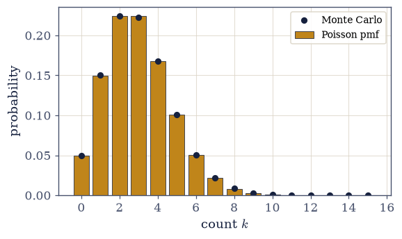
Fig. 404 The Poisson distribution for \(\lambda=3\), the law of rare events. The bars are the hand-built pmf \(\lambda^k e^{-\lambda}/k!\); the dark markers are a \(200{,}000\)-sample Monte Carlo with rng.poisson, in close agreement. The distinguishing feature is that the mean and the variance are both \(\lambda\) — so the spread of a counting experiment is the square root of its mean, the origin of \(\sqrt N\) counting noise in every detector.#
Exercise 7 — The binomial → Poisson limit (worked)#
Now the conceptual heart, worth taking slowly. Poisson is not an unrelated distribution; it is what the binomial becomes in the limit of many rare trials. Imagine a great many opportunities for an event, each individually very unlikely, with the average number of events held fixed: \(n\to\infty\), \(p\to0\), \(np=\lambda\) constant. A radioactive sample has \(\sim10^{23}\) nuclei (huge \(n\)), each with a tiny chance of decaying in the next second (tiny \(p\)), and a definite average decay rate (\(\lambda=np\)). In that limit the binomial \(\binom{n}{k}p^k(1-p)^ {n-k}\) converges term by term to \(\lambda^k e^{-\lambda}/k!\) Eq. 389 (Fig. 405); Feller, An Introduction to Probability Theory, Vol. I, Ch. VI, carries the term-by-term limit out in full. This is why decay counts, photon arrivals, and shot noise are all Poisson: each is a many-rare-events process.
The limit can be watched happening rather than asserted: hold \(\lambda=3\) fixed, let \(n\) grow through \(10\), \(30\) and \(1000\) with \(p=\lambda/n\) shrinking in lockstep, and the largest discrepancy from Poisson\((3)\) across all \(k\) falls off roughly as \(1/n\). The bars settle onto the Poisson curve as they go (Fig. 405).
Part a) Evaluate the binomial pmf with the binomial_pmf you wrote in Exercise 4 at those
three \(n\), and print at each one the numpy.max of the absolute difference from the Poisson
reference built with your Exercise 6 poisson_pmf.
Part b) Confirm that by \(n=1000\) the two agree to better than \(10^{-3}\) at every \(k\).
n=  10, p=λ/n=0.3000:  max |binomial − Poisson| = 4.28e-02
n=  30, p=λ/n=0.1000:  max |binomial − Poisson| = 1.20e-02
n=1000, p=λ/n=0.0030:  max |binomial − Poisson| = 3.37e-04
Validation 7#
✓ the binomial converges to the Poisson distribution in the rare-event limit [max|Δ| = 0.000336764 (rtol=1e-06, atol=0.001)]
True
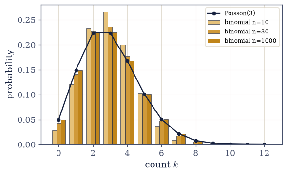
Fig. 405 The binomial becoming Poisson. With the mean held at \(\lambda=3\), the binomial pmf is shown for \(n=10\), \(30\), and \(1000\) trials (bars, lightening with \(n\)), each with \(p=\lambda/n\), against the Poisson\((3)\) limit (dark curve). As the trials grow many and individually rare, the binomial settles onto the Poisson, term by term — which is why a radioactive sample (\(n\sim10^{23}\) nuclei, tiny per-nucleus decay chance) counts Poisson.#
Exercise 8 — Expectation and variance: the Born-rule constructs (worked)#
Here is the payload of the notebook, and it is worth stating plainly. The expectation \(\langle A\rangle=\sum_i a_i P(a_i)\) and the variance \(\mathrm{Var}(A)=\langle A^2\rangle- \langle A\rangle^2\) Eq. 390 are not just the average and spread of a distribution. They are, exactly and without modification, the quantities quantum mechanics calls the expectation value of an observable and the square of its uncertainty \(\Delta A\). When Volume VI promotes observables to operators and writes \(\langle A\rangle=\langle\psi|\hat A| \psi\rangle\), the meaning is this same weighted average; and the Heisenberg uncertainty relation \(\Delta x\,\Delta p\ge\hbar/2\) is a statement about these very variances. We are not learning a classical preliminary to be discarded — we are learning the definitions QM uses, in a setting simple enough to see them whole.
The humblest observable is enough to see them whole. A fair die takes the values \(1\) through \(6\) with probability \(1/6\) each, so \(\langle A\rangle=3.5\) and \(\mathrm{Var}=35/12\approx 2.917\) — both checkable by hand, which is exactly why the die is the right specimen for definitions this important. The expectation value and the uncertainty are not quantum inventions; they are these elementary definitions, met again unchanged when observables become operators.
Part a) Compute \(\langle A\rangle\), \(\mathrm{Var}(A)\) and \(\Delta A=\sqrt{\mathrm{Var}}\)
for the fair die with the expectation and variance you wrote in Exercise 4, then report
the same three numbers for the Exercise 4 binomial.
Part b) Confirm the die’s \(\langle A\rangle=3.5\) and \(\mathrm{Var}=35/12\).
fair die:  ⟨A⟩ = 3.5  (= 3.5),  Var = 2.9167  (= 35/12),  ΔA = 1.7078
binomial:  ⟨k⟩ = 8.000,  Var = 4.800,  Δk = 2.191
these are the QM expectation value ⟨A⟩ and the uncertainty ΔA — Heisenberg bounds Δx·Δp
Validation 8#
✓ ⟨A⟩=Σ aP(a) and Var=⟨A²⟩−⟨A⟩² — the Born-rule expectation (3.5) and the uncertainty (35/12) [max|Δ| = 4.44089e-16 (rtol=1e-09, atol=1e-09)]
True
Exercise 9 — Variance of sums and the seed of sharpness (student)#
We end the conceptual arc with the fact that makes thermodynamics possible. For independent variables, variances add: \(\mathrm{Var}(X+Y)=\mathrm{Var}(X)+\mathrm{Var}(Y)\) Eq. 390. So if we average \(N\) independent, identically distributed measurements, the sum has variance \(N\sigma^2\) (it grows), but the mean — the sum over \(N\) — has variance \(\sigma^2/N\) (it shrinks). The relative fluctuation of the mean therefore falls as \(1/\sqrt N\). For \(N\sim10^{23}\) that is a relative spread of \(\sim10^{-12}\): the average becomes, for all practical purposes, a sharp number. This is the seed of why macrostates are sharp and thermodynamics is deterministic — the theme §5.3 develops in full.
The claim is easiest to see with dice again, whose single-die variance \(35/12\) you already computed in Exercise 8. Summing \(N\) of them and repeating the experiment many times gives both halves of the statement at once: \(\mathrm{Var}(\text{sum})/N\) should sit at that single-die value for every \(N\), while the relative spread of the mean should shrink by a factor of ten for each factor of a hundred in \(N\).
Part a) With numpy.random.default_rng, draw \(40{,}000\) samples of \(N\) dice for
\(N=1,10,100,1000\) and tabulate, for each \(N\), the variance of the sum divided by \(N\) beside
the relative standard deviation of the mean.
Part b) Confirm that \(\mathrm{Var}(\text{sum})=N\,\mathrm{Var}(\text{single})\) and that the relative fluctuation of the mean falls as \(1/\sqrt N\).
   N      Var(sum)/N      relative σ of the mean      1/√N
     1       2.904          0.48756                 0.48795
    10       2.899          0.15386                 0.15430
   100       2.914          0.04879                 0.04880
  1000       2.912          0.01542                 0.01543
Validation 9#
✓  variances of independent variables add: Var(sum) = N·Var(single)   [got 2.90449 vs expected 2.91667 (rtol=0.05, atol=1e-09)]
✓  the relative fluctuation of the mean falls as 1/√N   [got 0.100201 vs expected 0.1 (rtol=0.15, atol=1e-09)]
True
Exercise 10 — Monte Carlo estimation in practice (student)#
Finally, a glance ahead at the method that will carry this whole volume. Everything above we could compute exactly, but most physical systems are too complicated for that, and then we estimate probabilities and expectations by sampling Eq. 391. The estimate is itself a random quantity, and by the variance-of-the-mean result of Exercise 9 its error shrinks as \(1/\sqrt N\) — slow, but utterly general, and indifferent to the dimensionality that defeats other methods. Monte Carlo turns probability into a computational instrument, and from §5.4 it becomes the engine of statistical-mechanics simulation.
The classic demonstration is dart-throwing. Scatter points uniformly over the unit square and ask what fraction land inside the quarter circle of radius one: that fraction is the ratio of areas, \(\pi/4\), so four times it estimates \(\pi\). The estimate is a sample mean, so its error obeys the \(1/\sqrt N\) law of Exercise 9 — each factor of a hundred in \(N\) should cut the error by about ten.
Part a) Estimate \(\pi\) that way with numpy.random.default_rng at \(N=100\), \(10^4\) and
\(10^6\) points, printing the estimate and its error at each \(N\).
Part b) Confirm the errors fall as expected: report the ratio of successive errors and check the Monte Carlo estimate converges to \(\pi\).
  N=      100:  π ≈ 3.04000,  error = 0.10159
  N=   10,000:  π ≈ 3.15800,  error = 0.01641
  N=1,000,000:  π ≈ 3.14319,  error = 0.00160

error ratio over ×100 in N: 6.2 and 10.3  (≈10 = √100 each step)
Validation 10#
✓ the Monte Carlo estimate of π converges to the exact value [got 3.14161 vs expected 3.14159 (rtol=0.01, atol=1e-09)]
True
Notebook summary#
Probability turns the counts of §5.1 into the language physics speaks, and it hands quantum mechanics two of its central definitions ready-made.
From counts to probability Eq. 387: equally likely outcomes give \(P=\) favourable/total; all probabilities sum to one — the classical ancestor of \(\langle\psi| \psi\rangle=1\).
Conditional probability and Bayes Eq. 388: conditioning restricts the sample space (\(P(\text{sum}=8\mid\text{first}=5)=1/6\)); Bayes reverses it (\(P(A\mid\text{red})=2/3\)), as disciplined updating, not inference; independence multiplies (\(P(\text{both even})=1/4\)).
The physical distributions Eq. 389: the binomial (two-state system, \(\langle k\rangle=np\), verified against
scipy.stats), the multinomial and geometric, and the Poisson law of rare events (\(\langle k\rangle=\mathrm{Var}=\lambda\)), which the binomial becomes as \(n\to\infty,p\to0,np=\lambda\) (agreement to \(10^{-3}\) at \(n=1000\)).Expectation and variance — the Born-rule heart Eq. 390: \(\langle A\rangle= \sum a_iP(a_i)\) and \(\mathrm{Var}=\langle A^2\rangle-\langle A\rangle^2\) (\(3.5\) and \(35/12\) for a die) are the QM expectation value and the uncertainty \(\Delta A\) — Heisenberg is a variance statement. For independent variables variances add, so the mean of \(N\) sharpens as \(1/\sqrt N\), the seed of why macrostates are sharp.
Monte Carlo Eq. 391: probability as a computational tool, converging as \(1/\sqrt N\) — the engine of the physics from §5.4.
The distributions are the ones physical systems realize; the expectation and uncertainty, defined here in physics form, will be carried unchanged into Volume VI; and Monte Carlo is the instrument of everything that follows. What remains before the physics is the large-\(N\) limit — why, when \(N\sim10^{23}\), the most probable configuration does not merely win but utterly dominates. That is §5.3.
Outlook#
The large-\(N\) limit (§5.3). Stirling’s approximation, the law of large numbers, the central limit theorem, and why a macrostate’s overwhelming multiplicity makes thermodynamics deterministic.
The physics begins (§5.4 onward). Microstate probabilities become the Boltzmann distribution and entropy; Monte Carlo becomes the simulation method for the Ising model and beyond.
The Born rule (Volume VI). Probabilities as \(|\text{amplitude}|^2\), \(\langle A\rangle\) as \(\langle\psi|\hat A|\psi\rangle\), and the uncertainty principle as a variance relation — the constructs of this notebook made quantum.
Poisson processes (Volumes VI–VII). Photon counting and quantum optics, where the Poisson law of this notebook is the statistics of coherent light.
Cross-reference §5.1 (counting, the source of these probabilities) and Volume VI (the Born rule).