2.4 The Central-Force Problem and Orbits

Elementary Computational Physics

Volume II — Analytical Mechanics Notebook 2.4

Reducing two bodies to one radial coordinate: the effective potential, orbits as motion in 1-D, the Binet equation, and why only the inverse-square (and Hooke) law gives closed orbits.

Level · intermediate   •   Est. · 75–100 min

Raymond Amador v1.4.0  ·  2026-07-31  ·  CC BY 4.0 (text) / MIT (code)

Notebook overview

In §1.4 we integrated Kepler orbits directly in Cartesian coordinates and watched the ellipse close. This notebook is the analytical complement: instead of pushing \((x,y)\) forward in time, we use the two conserved quantities (energy and angular momentum) to collapse the whole two-dimensional problem onto a single radial coordinate, and then solve for the shape of the orbit itself.

The engine is one idea. Conservation of angular momentum (the rotational symmetry of §2.2; the cyclic angle of §2.3) lets us absorb the angular motion into an effective potential \(V_{\mathrm{eff}}(r)\), after which the radial coordinate moves exactly like a one-dimensional particle in that potential: the 1-D Hamiltonian motion of §2.3. Reading \(V_{\mathrm{eff}}(r)\) like a 1-D energy diagram tells us at a glance which orbits are circular (sit at the minimum), which are bound (oscillate between two turning points), and which escape. To get the geometric shape \(r(\varphi)\) we change variables to \(u=1/r\) and obtain the Binet equation, a linear oscillator equation whose solution is a conic section: the ellipse of §1.4, now derived rather than discovered.

You build the small toolkit yourself — V_eff and its two derivatives, the Binet right-hand side, and the analytic conic — while Setup supplies the given potential, a turning-point finder, and the 2-D Cartesian right-hand side of §1.4 for cross-checks. Then we put it to work: locating circular orbits and testing their stability, finding perihelion and aphelion as turning points, integrating the Binet equation and matching it to the analytic conic, animating the closed inverse-square ellipse, and finally animating the precessing rosette that appears the moment the force law departs from \(1/r^2\): the analytical sibling of the precession experiment of §1.4.

How to read the checks. Each exercise ends with a validation that compares a computed result to an expected physical fact. A ✗ does not by itself mean the physics is wrong: it means the output didn’t match what the check expected, which may be a real error, a different-but-valid convention (a sign, a unit, an array order), or simply too tight a tolerance. Treat a ✗ as a prompt to locate the discrepancy; passing is strong evidence of correctness, not proof.

Scope. This is a working review, not a textbook chapter. For the full derivation of the central-force reduction, the orbit equation, and Bertrand’s theorem, see Nolting, Theoretical Physics 2 [Nol16], Goldstein, Poole & Safko [GPS02] (ch. 3), and Landau & Lifshitz, Mechanics [LL76] (§III).

Theory in brief

Reduction to one body and one radial coordinate

A two-body system interacting through a potential that depends only on their separation reduces to a single fictitious particle of reduced mass \(\mu = m_1 m_2/(m_1+m_2)\) moving in the central potential \(V(r)\) about a fixed centre (§1.4). Because the force is central, the angular momentum

(148)\[\mathbf L = \mu\,\mathbf r \times \dot{\mathbf r}, \qquad L = \mu r^2 \dot\varphi = \text{const},\]

is conserved: this is the conserved charge of rotational symmetry (§2.2) and of the cyclic angle \(\varphi\) (§2.3). Its constancy confines the motion to a plane and fixes \(\dot\varphi = L/(\mu r^2)\), so the angular motion is no longer an independent unknown.

The effective potential: orbits as 1-D motion

Substituting \(\dot\varphi = L/(\mu r^2)\) into the energy \(E = \tfrac12\mu(\dot r^2 + r^2\dot\varphi^2) + V(r)\) removes \(\varphi\) entirely and leaves a purely radial energy equation,

(149)\[E = \tfrac12\mu\dot r^2 + V_{\mathrm{eff}}(r), \qquad V_{\mathrm{eff}}(r) = V(r) + \frac{L^2}{2\mu r^2}.\]

This is the conceptual heart of the chapter: the radial coordinate moves exactly like a one-dimensional particle of mass \(\mu\) in the potential \(V_{\mathrm{eff}}\) (a 1-D Hamiltonian system, §2.3). The extra term \(L^2/(2\mu r^2)\) is the centrifugal barrier (the angular-momentum cost of approaching the centre), and it is what keeps a particle with \(L\neq 0\) from falling in.

Circular orbits, turning points, and stability

Reading Eq. 149 as a 1-D energy diagram classifies every orbit:

• A circular orbit sits at a minimum of \(V_{\mathrm{eff}}\), where the inward force balances the centrifugal barrier. For the attractive inverse-square potential \(V=-GM\mu/r\) this gives

(150)\[\left.\frac{dV_{\mathrm{eff}}}{dr}\right|_{r_c}=0 \;\Longrightarrow\; r_c = \frac{L^2}{GM\mu^2},\]

and the orbit is stable when \(V_{\mathrm{eff}}''(r_c)>0\).

• A bound orbit (\(E<0\)) oscillates radially between two turning points, the roots of

(151)\[E = V_{\mathrm{eff}}(r) \qquad (\dot r = 0),\]

which are the perihelion \(r_{\min}\) and aphelion \(r_{\max}\).

• An unbound orbit (\(E\geq 0\)) has a single turning point and escapes: the scattering states that open §2.5.

The Binet equation and the conic-section orbit

To get the shape \(r(\varphi)\) rather than the timing, substitute \(u=1/r\) and use Eq. 148 to trade \(d/dt\) for \(d/d\varphi\). The radial equation becomes the Binet equation \(d^2u/d\varphi^2 + u = -\,\mu/(L^2u^2)\,F(1/u)\), where \(F=-dV/dr\). For the inverse-square force the right-hand side is constant,

(152)\[\frac{d^2u}{d\varphi^2} + u = \frac{GM\mu^2}{L^2},\]

a linear oscillator in \(\varphi\), and its solution is a conic section,

(153)\[u(\varphi)=\frac{GM\mu^2}{L^2}\bigl(1+e\cos\varphi\bigr), \qquad e=\sqrt{1+\frac{2EL^2}{G^2M^2\mu^3}}.\]

The eccentricity \(e\) sorts the orbits: \(e=0\) circle, \(0<e<1\) ellipse, \(e=1\) parabola, \(e>1\) hyperbola. Because the oscillator in Eq. 152 has unit angular frequency in \(\varphi\), the perihelion-to-aphelion apsidal angle is exactly \(\pi\): the orbit closes after one revolution. Bertrand’s theorem says only two force laws share this property: the inverse-square (\(\propto 1/r^2\)) and the Hooke (\(\propto r\)) law; every other central force precesses (§1.4).

---

Setup

We work in reduced units \(GM = 1\) and \(\mu = 1\), so the circular radius Eq. 150 is simply \(r_c = L^2\). What Setup holds is the given potential \(V(r)=-GM\mu/r\), a turning-point finder (a generic sign-change scan refined by brentq, bound to whatever effective potential it is handed), and the 2-D Cartesian right-hand side built from scratch in §1.4 and restated here for an independent cross-check. The notebook’s own machinery is not here: you write the effective potential V_eff and its slope dVeff_dr in Exercise 1, the curvature d2Veff_dr2 in Exercise 2, and the Binet right-hand side binet_rhs together with the analytic conic conic_orbit in Exercise 4.

The Setup below holds this notebook’s data and instruments — nothing you are asked to build. It is collapsed so the building stays yours; expand it whenever you want the details.

The geometry (a particle located by polar coordinates \((r,\varphi)\) about a fixed force centre) is sketched in Fig. 128.

Show code cell source

Hide code cell source

import numpy as np
from scipy.integrate import solve_ivp
from scipy.optimize import brentq
import matplotlib.pyplot as plt
from matplotlib.animation import FuncAnimation

from ecp import draw, mechanics, validate
from ecp.animate import show

GM = 1.0  # data: reduced units — GM = μ = 1 throughout
MU = 1.0


# instrument: the *given* central potential, not a method — the inverse-square
# law is this notebook's input, and the lesson is what the reduction does with
# it, not writing down $-GM\mu/r$.
def V(r):
    """Attractive inverse-square potential energy V(r) = −GM·μ/r.

    Parameters
    ----------
    r : float or numpy.ndarray
        Radius.

    Returns
    -------
    float or numpy.ndarray
        The potential energy.
    """
    return -GM * MU / r


# instrument: a root-bracketing adapter — the sign-change scan and its Brent
# refinement live in `ecp.mechanics`, and this only binds them to the effective
# potential, the `V_eff` you build in Exercise 1 (Python looks the name up at
# call time, not at definition time).
def turning_points(E, L, r_lo=1e-3, r_hi=1.0e3, n_scan=200_000):
    """Radial turning points: the roots of E − V_eff(r) (eq-turning).

    Two roots bound a closed orbit; found by a sign-change scan plus Brent
    refinement.

    Parameters
    ----------
    E : float
        Orbit energy.
    L : float
        Angular momentum.
    r_lo, r_hi : float, optional
        Search bounds.
    n_scan : int, optional
        Scan resolution.

    Returns
    -------
    numpy.ndarray
        The turning-point radii.
    """
    return mechanics.turning_points(E, lambda rr: V_eff(rr, L), r_lo, r_hi, n_scan)


# built from scratch in §1.4 (Exercise 1, there called `rhs`); restated here as
# an instrument, so Exercise 7's cross-check owes nothing to the reduction.
def cartesian_rhs(_t, s):
    """2-D Newtonian central-force state derivative (reused from §1.4)."""
    x, y, vx, vy = s
    r3 = (x * x + y * y) ** 1.5
    return [vx, vy, -GM * MU * x / r3, -GM * MU * y / r3]

Exercise 1 — The effective potential

Everything in this chapter is read off one curve. The effective potential Eq. 149 superposes the attractive well \(V(r)=-GM\mu/r\) (which pulls inward) on the repulsive centrifugal barrier \(L^2/(2\mu r^2)\) (which the conserved angular momentum Eq. 148 erects near the origin). Their sum has a well with a single minimum, and that shape dictates every orbit. Larger \(L\) raises a higher barrier and pushes the minimum outward. Setting \(dV_{\mathrm{eff}}/dr=0\) in Eq. 150 puts that minimum at the circular radius \(r_c=L^2/(GM\mu^2)\), which in reduced units is simply \(r_c=L^2\) — the prediction the last step checks.

1. Write V_eff(r, L), the effective potential Eq. 149: the given V(r) plus the centrifugal barrier \(L^2/(2\mu r^2)\). Write this one yourself — the implementation is the lesson; every result in this notebook is read off this one curve.

2. Write dVeff_dr(r, L), its analytic first derivative \(GM\mu/r^2 - L^2/(\mu r^3)\), which vanishes at a circular orbit Eq. 150.

3. Plot \(V_{\mathrm{eff}}(r)\) for several angular momenta \(L\), on a common axis, marking the attractive well and the centrifugal barrier. The result is shown in Fig. 129.

4. Confirm that the well’s minimum sits at \(r_c=L^2\) by checking \(dV_{\mathrm{eff}}/dr=0\) there, for each \(L\).

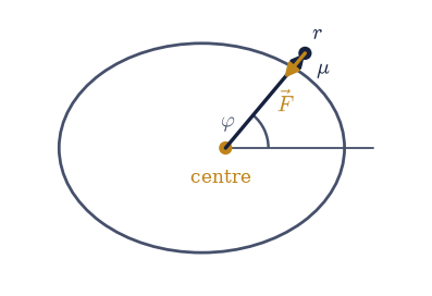
Fig. 128 Central-force geometry: the reduced particle of mass \(\mu\) (the relative coordinate of the two bodies) is located by polar coordinates \((r,\varphi)\) about the fixed force centre (amber) — radius \(r\) and azimuth \(\varphi\) from the polar axis; the central force \(\mathbf F=-(dV/dr)\,\hat{\mathbf r}\) points along the radius, so the angular momentum \(L=\mu r^2\dot\varphi\) is conserved and the motion stays in this plane.

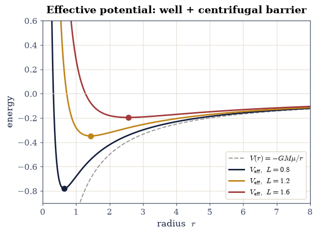
Fig. 129 The effective potential \(V_{\mathrm{eff}}(r)=-GM\mu/r+L^2/(2\mu r^2)\) (reduced units \(GM=\mu=1\)) for three angular momenta \(L\): the attractive Kepler well (dashed) plus the repulsive centrifugal barrier \(L^2/(2\mu r^2)\) produce a well whose minimum (dot) is the circular-orbit radius \(r_c=L^2\); larger \(L\) raises a higher barrier and pushes the minimum outward.

Validation 1 — the circular orbit sits at the \(V_{\mathrm{eff}}\) minimum

The minimum of \(V_{\mathrm{eff}}\) is where the radial force Eq. 150 vanishes. In reduced units that predicts \(r_c = L^2\) for every \(L\), so the dVeff_dr you wrote in Part 2, evaluated at \(r_c=L^2\), must be zero.

✓  circular orbit sits at the V_eff minimum r_c=L²=0.64  (L=0.8)   [got 0 vs expected 0 (rtol=1e-06, atol=1e-06)]
✓  circular orbit sits at the V_eff minimum r_c=L²=1.44  (L=1.2)   [got 0 vs expected 0 (rtol=1e-06, atol=1e-06)]
✓  circular orbit sits at the V_eff minimum r_c=L²=2.56  (L=1.6)   [got 0 vs expected 0 (rtol=1e-06, atol=1e-06)]

Exercise 2 — Circular orbits and their stability

A minimum of \(V_{\mathrm{eff}}\) is a circular orbit; whether it is stable depends on the curvature there. A small radial nudge sees the local quadratic \(V_{\mathrm{eff}}\approx V_{\mathrm{eff}}(r_c)+\tfrac12 V_{\mathrm{eff}}''(r_c)(r-r_c)^2\), so the orbit oscillates back (stable) when \(V_{\mathrm{eff}}''(r_c)>0\) and runs away (unstable) when it is negative. The inverse-square law gives a genuine well, so its circular orbits are stable: the reason planets keep their orbits. Differentiating Eq. 149 twice gives that curvature in closed form, \(V_{\mathrm{eff}}''(r) = -2GM\mu/r^3 + 3L^2/(\mu r^4)\).

1. Write d2Veff_dr2(r, L), the second derivative above: the sign of this one number decides whether a circular orbit survives a nudge.

2. Take \(L=1.2\), locate the circular radius \(r_c=L^2\) from Eq. 150, and evaluate the curvature \(V_{\mathrm{eff}}''(r_c)\) there.

3. Plot the V_eff you wrote in Exercise 1 with the circular orbit marked at the bottom of the well and the local parabola overlaid, as in Fig. 130.

circular radius r_c = 1.4400,  V_eff''(r_c) = 0.3349  (>0 ⇒ stable)

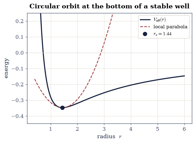
Fig. 130 Stability of the inverse-square circular orbit: \(V_{\mathrm{eff}}(r)\) for \(L=1.2\) (solid) with the circular orbit (dot) at the minimum \(r_c=L^2=1.44\); the dashed parabola is the local quadratic approximation \(V_{\mathrm{eff}}(r_c)+\tfrac12 V_{\mathrm{eff}}''(r_c)(r-r_c)^2\), whose upward curvature \(V_{\mathrm{eff}}''(r_c)>0\) means a radial nudge oscillates back — the orbit is stable.

Validation 2 — the inverse-square circular orbit is stable

Stability is the single inequality \(V_{\mathrm{eff}}''(r_c)>0\): the well curves upward, so the orbit is a stable equilibrium of the radial 1-D motion.

✓  the inverse-square circular orbit is stable (V_eff''(r_c) > 0)   [V_eff''(r_c) = 0.3349]

True

Exercise 3 — Turning points and the radial 1-D picture

For a bound orbit (\(E<0\)) the radial coordinate is trapped in the well and bounces between two turning points (the perihelion \(r_{\min}\) and aphelion \(r_{\max}\)), exactly where the horizontal energy line \(E\) cuts the \(V_{\mathrm{eff}}\) curve, \(\dot r=0\) in Eq. 151. This is the radial motion read straight off the 1-D energy diagram. The conic solution Eq. 153 predicts these turning points analytically as \(a(1\mp e)\) with semi-major axis \(a=-GM\mu/(2E)\): a clean cross-check.

1. Take \(L=1\) and \(E=-0.32\) (a bound orbit). Find \(r_{\min},r_{\max}\) as the roots of Eq. 151 with the Setup’s turning_points — a sign-change scan refined by scipy.optimize.brentq, which brackets the roots of \(E-V_{\mathrm{eff}}\) using the V_eff you wrote in Exercise 1.

2. Plot that same \(V_{\mathrm{eff}}(r)\) with the energy line \(E\) and the two turning points marked (Fig. 131), shading the classically allowed region \(E\geq V_{\mathrm{eff}}\).

turning points: r_min = 0.625000, r_max = 2.500000
conic predicts: a(1−e) = 0.625000, a(1+e) = 2.500000
eccentricity e = 0.6000, semi-major axis a = 1.5625

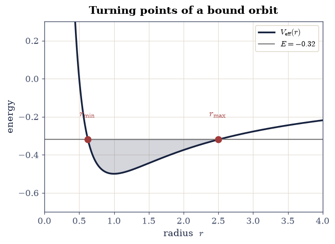
Fig. 131 The bound radial orbit as 1-D motion (\(L=1\), \(E=-0.32\)): the energy line \(E\) (grey) cuts the effective potential \(V_{\mathrm{eff}}(r)\) at the perihelion \(r_{\min}\) and aphelion \(r_{\max}\) (dots), the turning points where \(\dot r=0\); the radial coordinate oscillates across the shaded classically allowed region \(E\ge V_{\mathrm{eff}}\), while the centrifugal barrier blocks the origin.

Validation 3 — turning points equal the conic’s \(a(1\mp e)\)

The turning points found numerically from \(E=V_{\mathrm{eff}}\) must coincide with the perihelion and aphelion of the analytic conic Eq. 153, \(a(1-e)\) and \(a(1+e)\): two independent routes to the same two radii.

✓  turning points equal a(1∓e) from the conic   [max|Δ| = 3.7792e-13 (rtol=1e-06, atol=1e-09)]

True

Exercise 4 — The Binet equation reproduces the conic

The energy diagram gives the radial range but not the orbit’s shape. For that we switch from time to angle: with \(u=1/r\), the radial equation becomes the linear Binet oscillator Eq. 152, whose solution is the conic Eq. 153. Rather than quote that solution we integrate the Binet ODE numerically from perihelion and check that it traces the analytic conic: a derivation made concrete. Both sides of that check are written here — the oscillator as a first-order system \([u', \, GM\mu^2/L^2 - u]\), and the closed form \(u(\varphi)=(1+e\cos\varphi)/p\) with semi-latus rectum \(p=L^2/(GM\mu^2)\) that it must reproduce.

1. Write binet_rhs(phi, y, L), the inverse-square Binet equation Eq. 152 as a first-order system in \(y=[u,\,u']\) (the angle argument is unused — solve_ivp requires it). Write this one yourself — the implementation is the lesson: this two-line right-hand side is the orbit equation.

2. Write conic_orbit(L, e), returning the analytic \(u(\varphi)\) of Eq. 153 as a callable: the yardstick the integration is judged by.

3. Use the same orbit (\(L=1\), \(E=-0.32\), hence \(e\approx0.6\)). Start at perihelion: \(u(0)=(1+e)/p\), and \(u'(0)=0\). Integrate Eq. 152 over \(\varphi\in[0,2\pi]\) with scipy.integrate.solve_ivp (DOP853, rtol=1e-11, atol=1e-13) on a dense phi-grid.

4. Overlay the integrated \(u(\varphi)\) on the analytic conic, and plot the corresponding orbit \(r(\varphi)\) in the plane (Fig. 132).

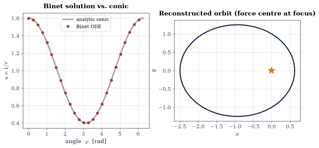
Fig. 132 The Binet equation yields the conic orbit (\(L=1\), \(e=0.6\)). Left: \(u(\varphi)=1/r\) from numerically integrating the linear Binet equation Eq. 152 (markers) lies on the analytic conic Eq. 153 (line). Right: the reconstructed orbit \(r(\varphi)\) in the plane is a closed ellipse with the force centre (amber) at one focus, perihelion on the right, aphelion on the left.

Validation 4 — the Binet integration is the conic

The numerically integrated Binet solution must match the closed-form conic Eq. 153 pointwise: same orbit, one route analytic and one numerical.

✓  the Binet equation yields the conic-section orbit   [max|Δ| = 4.11708e-11 (rtol=1e-06, atol=1e-09)]

True

Exercise 5 — Apsidal angle and orbit closure (worked animation)

Why does the Kepler ellipse close? Because the Binet oscillator Eq. 152 advances \(u\) through exactly one full cycle as \(\varphi\) goes from perihelion to perihelion: the angle from perihelion to aphelion (the apsidal angle) is exactly \(\pi\), so after \(2\pi\) the orbit returns to its start. The apsidal line (the major axis joining perihelion and aphelion through the focus) never rotates. This is the analytic statement of what §1.4 found by integration. The apsidal geometry is sketched in Fig. 133; the animation traces the closed ellipse, and the validation measures the apsidal angle of the animated orbit, not the animation object.

This is the worked animation; you build the second in Exercise 6. The orbit it draws is the analytic conic u_of_phi returned by your Exercise 4 conic_orbit.

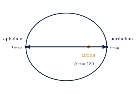
Fig. 133 Apsidal geometry of a bound orbit: the force centre (amber) sits at one focus; the particle’s radius reaches its minimum \(r_{\min}\) at perihelion (right) and its maximum \(r_{\max}\) at aphelion (left), joined by the dashed apsidal line through the focus. For the inverse-square law the apsidal angle from perihelion to aphelion is exactly \(\Delta\varphi=180^\circ\), so the orbit closes and the apsidal line stays fixed.

measured apsidal angle (perihelion → aphelion) = 179.955°

Once Loop Reflect

Fig. 134 Animation of the closed inverse-square orbit (\(L=1\), \(e=0.6\)): the particle (blue) traces an ellipse with the force centre (amber star) at one focus and the fixed apsidal line (dashed) joining perihelion and aphelion. The orbit closes after one revolution because the apsidal angle is exactly \(180^\circ\) — the analytic counterpart of the closure measured by integration in §1.4.

Validation 5 — the apsidal angle is 180° (the orbit closes)

The defining property of the inverse-square orbit: the angle swept from perihelion to aphelion is \(180^\circ\). Measured from the animated orbit data, it must equal \(180^\circ\) to within the angular grid resolution: the orbit closes.

✓  inverse-square apsidal angle is 180° (closed orbit)   [got 179.955 vs expected 180 (rtol=1e-06, atol=0.5)]

True

Exercise 6 — Precession under a modified force law (student-implemented animation)

The closure of the orbit is a knife-edge property of the \(1/r^2\) law. Add even a small extra term and the apsidal angle stops being \(180^\circ\): the ellipse fails to close, and instead its apsidal line slowly precesses, tracing a rosette. We model this with a relativistic-like correction to the Binet equation,

\[\frac{d^2u}{d\varphi^2} + u = \frac{GM\mu^2}{L^2} + \beta\,u^2,\]

the same \(u^2\) term that produces Mercury’s perihelion advance in general relativity (a forward link to “Outlook”). This is the analytical sibling of Exercise 7 of §1.4, which integrated a modified force law in Cartesian coordinates and watched the same rosette appear.

This is the student-implemented animation: the modified dynamics is given; you build the player and measure the precession.

1. Integrate the modified Binet equation above with scipy.integrate.solve_ivp (DOP853) over several orbits (use \(\beta=0.1\), \(L=1\), and the unperturbed perihelion of your Exercise 4 conic_orbit at \(e=0.6\) as the start), storing \(u(\varphi)\). The right-hand side is the binet_rhs you wrote in Exercise 4 with the extra \(\beta u^2\) term.

2. Build the animation of the precessing rosette \(r(\varphi)=1/u\) in the plane, with the slowly rotating apsidal line (there are many valid ways to draw it), then plt.close(fig) and end with ecp.animate.show(anim).

3. Detect successive perihelia (interior maxima of \(u\) on the dense grid) and measure the precession per orbit: the perihelion-to-perihelion angle minus \(360^\circ\).

A ✗ on the final check is about the perihelion detection or the orbit data, not the drawing: any correct animation of the same data is fine. If it fails, check that consecutive \(u\)-maxima are being found on a finely sampled grid.

perihelion-to-perihelion angle = 409.64°
precession per orbit = +49.64°  (β=0.1)

Once Loop Reflect

Fig. 135 Animation of a precessing rosette orbit under the modified Binet law \(u''+u=GM\mu^2/L^2+\beta u^2\) (\(\beta=0.1\), \(L=1\), \(e=0.6\)): the extra \(u^2\) term breaks the inverse-square closure, so each successive perihelion advances and the apsidal line (dashed, drawn to the current perihelion) slowly rotates, tracing a rosette. This is the analytical sibling of the modified-force precession of §1.4.

Validation 6 — the modified force law precesses

The signature of any non-inverse-square central force: the orbit does not close, so the precession per orbit is nonzero. We require a clear, measurable advance (well above a degree) from the animated orbit’s perihelia.

✓  the modified force law precesses the orbit   [precession = +49.64°/orbit]

True

Exercise 7 — Cross-check: full 2-D integration conserves \(E\) and \(L\)

Our whole reduction rested on two conserved quantities. As an independent close, we drop back to the unreduced picture and integrate the orbit in Cartesian coordinates with the Newtonian force (the right-hand side from §1.4), making no use of \(V_{\mathrm{eff}}\) or Binet. If the analysis is right, the Cartesian orbit must (i) conserve the energy \(E\) and angular momentum \(L\) that Eq. 149 and Eq. 148 assumed constant, and (ii) trace the same conic Eq. 153 we derived.

1. Launch the same orbit from perihelion (\(x=r_{\min}\), \(v_y=L/r_{\min}\)) and integrate the Setup’s cartesian_rhs with scipy.integrate.solve_ivp (DOP853) over several periods.

2. Track \(E(t)=\tfrac12 v^2 - GM\mu/r\) and \(L(t)=x v_y - y v_x\) and confirm both are conserved; overlay the Cartesian orbit on the analytic conic from your Exercise 4 conic_orbit (Fig. 136).

E: -0.320000 → -0.320000   L: 1.000000 → 1.000000

Fig. 136 Independent 2-D cross-check (\(L=1\), \(E=-0.32\)). Left: the orbit integrated in Cartesian coordinates with the Newtonian inverse-square force (dashed) lies on the analytic conic Eq. 153 (solid), force centre (amber) at the focus. Right: the energy \(E\) and angular momentum \(L\) stay constant along the trajectory — the two conserved quantities the effective-potential reduction relies on.

Validation 7 — energy and angular momentum are conserved

The two constants the reduction assumed must hold along the fully independent 2-D trajectory: \(E\) and \(L\) may drift only at the integrator’s tolerance.

✓  energy conserved (2-D integration)   [max relative drift = 1.7353e-10 (limit 1e-06)]
✓  angular momentum conserved (2-D integration)   [max relative drift = 7.39275e-11 (limit 1e-06)]

True

Exercise 8 — What makes an orbit precess: an exactly solvable case (worked)

Exercise 6 showed that a modified force law precesses the orbit. We can now make that quantitative, because there is a perturbation the effective potential solves exactly. Add a small extra inverse-square term to the potential,

\[V(r)=-\frac{k}{r}-\frac{\beta}{r^2},\]

which contributes an inverse-cube force. The point is what it does to the effective potential: the extra \(-\beta/r^2\) merges with the centrifugal term \(L^2/2\mu r^2\) into a single \(1/r^2\) piece with coefficient \((L^2/2\mu-\beta)\) Eq. 149. The radial problem is therefore identical to Kepler’s but with a shifted angular-momentum barrier, so it can be solved in closed form. The apsidal angle — perihelion to aphelion — becomes

\[\Phi=\frac{\pi}{\sqrt{1-2\beta/L^2}},\]

and the perihelion advances by \(2(\Phi-\pi)=2\pi\!\left(1/\sqrt{1-2\beta/L^2}-1\right)\) each orbit. Because the case is exactly solvable, this is not a small-\(\beta\) approximation; it is the precise rate, and our integrated orbit must match it at any \(\beta\) (Fig. 137).

This exercise (worked). For a reference orbit (\(L=1\), \(e=0.4\), so \(a=1/(1-e^2)\)) with \(\beta=0.05\):

1. Integrate the perturbed motion in Cartesian coordinates with scipy.integrate.solve_ivp (DOP853), locating each perihelion with a solve_ivp event on \(\mathbf r\cdot\mathbf v=0\).

2. Measure the per-orbit advance of the perihelion direction (the change in \(\operatorname{atan2}(y,x)\) at successive perihelia, via numpy.unwrap).

3. Confirm it matches the exact apsidal-angle formula.

perturbation V=-k/r-β/r², β=0.05, L=1.0:
  measured precession = 19.4733°/orbit
  exact formula 2π(1/√(1−2β/L²)−1) = 19.4733°/orbit

Validation 8 — precession matches the exact apsidal-angle formula

✓  a small departure from 1/r² makes the orbit precess, at the rate the apsidal-angle formula predicts   [got 0.339874 vs expected 0.339874 (rtol=0.01, atol=1e-09)]

True

Fig. 137 The precessing rosette under \(V=-k/r-\beta/r^2\) (\(\beta=0.05\)), over six orbits. The added \(-\beta/r^2\) term shifts the centrifugal barrier, so the apsidal angle is no longer \(180^\circ\) and the perihelion (red dots) advances a fixed amount each orbit — here \(19.5^\circ\), matching the exact formula \(2\pi(1/\sqrt{1-2\beta/L^2}-1)\) to numerical precision. Any departure from the inverse-square law turns the perihelion; this one we can predict exactly.

Exercise 9 — The general-relativistic term, and Mercury’s anomaly (student)

The mechanism is general: any departure from \(1/r^2\) precesses the orbit. Exercise 6 used the \(\beta u^2\) correction to the Binet equation — an inverse-fourth-power force — and this is the exact form general relativity adds. The capstone of Volume IV (§4.8) derives it: GR modifies the orbit equation by precisely \(3GM u^2/c^2\), and the resulting precession is \(6\pi GM/[a(1-e^2)c^2]\) per orbit. Here we confirm that the GR-form term, with its physical coefficient, reproduces that prediction — and then we lay out where Mercury’s famous number actually comes from.

This exercise (student).

1. Reuse the modified Binet right-hand side binet_rhs_mod from Exercise 6 with the relativistic coefficient \(\beta=3GM/c^2\), in toy units with \(c=100\) (so the perturbation is small), integrating with scipy.integrate.solve_ivp (DOP853) and a solve_ivp event on \(du/d\varphi=0\) to pin each perihelion.

2. Confirm the measured precession matches \(6\pi GM/[a(1-e^2)c^2]\).

GR-form term β=3GM/c² (c=100):
  measured precession   = 1.886408e-03 rad/orbit
  formula 6πGM/(a(1−e²)c²) = 1.884956e-03 rad/orbit

Validation 9 — the GR-form term gives the GR precession formula

✓  the inverse-fourth (general-relativistic) term precesses the orbit
✓  the GR-form term gives exactly the precession 6πGM/(a(1−e²)c²)   [got 0.00188641 vs expected 0.00188496 (rtol=0.01, atol=1e-09)]

True

Mercury’s perihelion: an honest accounting

We can now state the famous puzzle truthfully, which matters, because it is easy to tell it wrong. Mercury’s perihelion advances by about \(574''\) per century relative to the fixed stars. Where does it come from?

• An isolated Sun–Mercury system would not precess at all. By the closure of the inverse-square orbit (§1.4, the conserved Laplace–Runge–Lenz vector), a pure two-body Kepler ellipse is perfectly closed. The naive Sun–Mercury model predicts zero advance.

• About \(531''\)/century comes from Newtonian gravitational tugs of the other planets, which perturb Mercury away from a pure \(1/r^2\) field — and, by the mechanism of this notebook, any such departure makes the orbit precess.

• That leaves a residual of about \(43''\)/century that no Newtonian effect explains. For decades this stubborn remainder was the outstanding anomaly of celestial mechanics.

The resolution is the term we just integrated. General relativity adds an inverse-fourth-power correction to the gravitational force — precisely the \(3GMu^2/c^2\) form above — and it supplies exactly the missing \(43''\) per century. The capstone §4.8 carries out that calculation with the physical constants and lands on the observed number. The point worth holding onto is that the reader now has, in the very code of this notebook, everything needed to see the puzzle: an isolated orbit closes, any non-\(1/r^2\) term turns it, and a \(1/r^4\) term turns it at a computable rate. General relativity supplies the missing piece, and §4.8 collects it.

Notebook summary

• The effective potential \(V_{\rm eff}(r)=V(r)+L^2/2\mu r^2\) — one line of physics, written out — circular orbits and their stability, and the turning points that frame the radial 1-D picture.

• The Binet equation reproducing the Kepler conic; the apsidal angle and orbit closure; precession under a modified force law; and a full 2-D integration conserving both energy and angular momentum.

• What makes an orbit precess. An exactly solvable \(-\beta/r^2\) perturbation shifts the centrifugal barrier and advances the perihelion by exactly \(2\pi(1/\sqrt{1-2\beta/L^2}-1)\); the general-relativistic \(3GMu^2/c^2\) term gives \(6\pi GM/[a(1-e^2)c^2]\). An isolated Kepler orbit (§1.4) does not precess; planetary tugs supply most of Mercury’s \(574''\)/century, and the residual \(43''\) is the relativistic piece collected in the capstone §4.8.

Outlook

• Scattering states (\(E>0\)). An unbound orbit is a hyperbola with a single turning point; the angle through which it is deflected, as a function of the impact parameter, is the central-force scattering problem: the direct sequel in §2.5.

• The Laplace–Runge–Lenz vector. The inverse-square orbit conserves one more vector quantity, \(\mathbf A = \mathbf p\times\mathbf L - GM\mu^2\,\hat{\mathbf r}\), which points along the apsidal line and so explains why it does not precess: the “hidden” symmetry hinted at in §2.2.

• Mercury’s perihelion. The \(\beta u^2\) term of Exercise 6 is exactly the form of the general-relativistic correction; with the physical coefficient \(3GM/c^2\) it predicts Mercury’s observed \(43''\) per century.

• The other closed orbit. Bertrand’s theorem leaves only one more force law with closed orbits (the isotropic Hooke oscillator \(V\propto r^2\)) whose ellipse is centred on, not focused at, the force centre.

References

[GPS02]

Herbert Goldstein, Charles P. Poole, and John L. Safko. Classical Mechanics. Pearson, 3 edition, 2002.

[LL76]

L. D. Landau and E. M. Lifshitz. Mechanics. Volume 1 of Course of Theoretical Physics. Butterworth–Heinemann, 3 edition, 1976.

[Nol16]

Wolfgang Nolting. Theoretical Physics 2: Analytical Mechanics. Springer, 2016.

Take this notebook with you

Use the download button (↓) in the toolbar above to save this notebook and run it yourself. The published notebooks ship without worked solutions; if you would like the reference solutions — to teach from or to check your own work — get in touch: hello@ramador.me.