


0.14 Partial Differential Equations: Stability, Explicit and Implicit#
Notebook overview#
Volume 0 has so far stopped at ordinary differential equations. The standard computational-physics texts do not stop there: Pang’s An Introduction to Computational Physics devotes its chapter 7 to partial differential equations, Newman’s Computational Physics reaches them in chapter 9 immediately after his ODE chapter, and Landau, Páez & Bordeianu spend chapters 19 to 23 on them. Brigham Young’s computational-physics sequence runs an entire separate course on PDEs for the same reason: the ODE material was the prerequisite, not the destination. This notebook is that continuation, and it is the last methods notebook of Volume 0.
I want to be honest about what it is not. It is not a repair. Every propagator elsewhere in this course was chosen to be unconditionally stable, so nothing here fixes a wrong number: §3.8 animates an analytic travelling wave rather than marching one, §6.13 propagates wave packets with the split-step Fourier method, and §8.16 uses Crank–Nicolson, which its own prose calls unconditionally unitary by construction. Those were good choices. They were also, until now, silent ones: search the rest of the course for “CFL”, “Courant”, “von Neumann stability” or “amplification factor” and nothing comes back. The job of this notebook is to make the choice visible rather than lucky, so that a reader who later writes a marching scheme of their own knows which question to ask before pressing run.
The thread from §0.7 is unbroken. There, the test equation \(y'=-ky\) made explicit Euler explode unless \(h \le 2/k\), and the cure was to go implicit. Here a PDE becomes a large stiff ODE system the moment we discretize space, its stiffness set by the grid spacing, and the same two moves return in their PDE dress: an explicit scheme with a hard step ceiling, and implicit schemes with none. The elliptic case needs no marching at all and is already solved in §3.4 by relaxation; we cite that notebook rather than rebuild it, and we do find that its Jacobi sweep and our explicit diffusion step are literally the same line of code.
Units are reduced throughout: the diffusivity \(D\), the wave speed \(c\), and the rod length \(L\) are all set to \(1\), so lengths are measured in rod lengths and times in diffusion times \(L^2/D\). No physical constants enter.
How to read the checks. Each exercise ends with a
validatecall against an independent fact: a closed-form solution, a predicted amplification factor, a convergence order. A ✓ is strong evidence; a ✗ is a prompt to locate the discrepancy (a real error, a convention difference, or too tight a tolerance), not a verdict.
Scope. A working introduction, not a course in numerical PDEs. The standard references are Press et al., Numerical Recipes, ch. 20 [PTVF07], and for the analysis proper, LeVeque’s Finite Difference Methods for Ordinary and Partial Differential Equations.
Theory in brief#
Three types, and why the type picks the method#
A second-order linear PDE in two independent variables can always be written
and the sign of the discriminant \(\Delta\) splits every such equation into exactly three families, each with its own physics and its own numerics:
Elliptic (\(\Delta < 0\)): Laplace and Poisson, \(\nabla^2\varphi = -\rho/ \varepsilon_0\). There is no time variable and no marching direction; every interior value is fixed by the boundary all at once, which is why the method is a global solve, either iterative relaxation or a sparse factorization (§3.4).
Parabolic (\(\Delta = 0\)): the diffusion (heat) equation Eq. 81. One variable is time, so the problem is an initial-value problem in \(t\) and a boundary-value problem in \(x\): we march. Diffusion smooths, damping short wavelengths hardest.
Hyperbolic (\(\Delta > 0\)): the wave equation Eq. 86. We march again, but nothing is damped; information travels along the characteristics \(x \pm ct\) at the finite speed \(c\), and that finite speed will turn out to set the step ceiling.
The classification is not taxonomy for its own sake. It says whether there is a marching direction at all, and once there is one, the step along it is no longer ours to choose freely.
The method of lines: a PDE is a stiff ODE system#
Take the diffusion equation on \(0 \le x \le L\) with fixed (Dirichlet) ends,
Sample \(u\) on a uniform grid \(x_j = j\,\Delta x\) and replace the spatial derivative by the three-point second difference, the 1-D sibling of the five-point stencil of §3.4,
Space is now discrete but time is still continuous, which leaves one ODE per interior grid point, \(\dot u_j = D(u_{j+1}-2u_j+u_{j-1})/\Delta x^2\). This is the method of lines, and it means the entire vocabulary of §0.7 applies unchanged. In particular, the matrix of that linear system has eigenvalues \(\lambda_m = -(4D/\Delta x^2)\sin^2(m\pi\Delta x/2L)\), whose magnitudes run up to \(4D/\Delta x^2\): refining the grid makes the system stiffer, quadratically. Explicit Euler on a decay rate \(k\) needed \(h \le 2/k\) (Eq. 47), so with \(k = 4D/\Delta x^2\) the step ceiling \(\Delta t \le \Delta x^2/(2D)\) is already visible before we write a line of code.
FTCS and the amplification factor#
Applying explicit Euler in time to that system gives the FTCS scheme (forward in time, centred in space),
where the dimensionless diffusion number \(C\) is the only combination of \(D\), \(\Delta t\) and \(\Delta x\) the scheme knows about. Von Neumann’s analysis asks what the scheme does to a single Fourier mode. Substituting the trial form \(u_j^{\,n} = A^n e^{\mathrm i\theta j}\), with \(\theta = k\,\Delta x\) the phase advance per cell (only \(|\theta| \le \pi\) is representable on the grid, the Nyquist limit of §0.6), the second difference contributes \(e^{\mathrm i\theta} - 2 + e^{-\mathrm i\theta} = 2(\cos\theta - 1) = -4\sin^2(\theta/2)\), and every power of \(A\) cancels but one:
\(A\) is the factor by which one step multiplies that mode, so the scheme is stable exactly when no mode grows, \(|A(\theta)| \le 1\) for every representable \(\theta\). Since \(\sin^2\) reaches \(1\) at \(\theta = \pi\) (the sawtooth mode \(+1, -1, +1, \dots\), one wavelength per two cells), the binding requirement is \(|1 - 4C| \le 1\), that is
Two things about this bound deserve emphasis. It is quadratic in \(\Delta x\), so halving the grid spacing quarters the largest legal step: a fine grid is expensive twice over. And past the bound the sawtooth grows by \(|1-4C|\) per step while flipping sign, so the failure is not a gentle loss of accuracy but an exponential eruption at the shortest wavelength the grid can hold. The analysis assumes constant coefficients and ignores the boundaries, which makes it a local criterion; in practice it is the working tool, and for the linear problems here it is exact.
The wave equation and the CFL condition#
The hyperbolic case is
whose free-space solution is d’Alembert’s, \(u(x,t) = \tfrac12[f(x-ct) + f(x+ct)]\) for initial displacement \(f\) released from rest. Centring the second difference in both variables gives the three-level leapfrog scheme
with \(r\) the Courant number. Von Neumann now yields a quadratic for the per-step factor \(\xi\), namely \(\xi^2 - 2\big[1 - 2r^2\sin^2(\theta/2)\big]\xi + 1 = 0\). The product of its two roots is \(1\), so either both roots sit on the unit circle (nothing grows and nothing damps, exactly as a wave should behave) or one of them lies outside it. The roots stay on the circle precisely when the bracket has magnitude at most one, which for all \(\theta\) means
the Courant–Friedrichs–Lewy (CFL) condition. It has a reading that needs no algebra: in one step the scheme gathers information from one cell on either side, so its numerical domain of dependence spans \(\pm\Delta x\), while the true solution at that point depends on data within \(\pm c\,\Delta t\). If \(c\,\Delta t > \Delta x\) the scheme is computing an answer that depends on data it never looked at, and no amount of arithmetic can rescue that. Notice the contrast with diffusion: the CFL bound is linear in \(\Delta x\), which is why explicit schemes remain perfectly practical for wave problems.
Implicit schemes: backward Euler and Crank–Nicolson#
The cure is the one §0.7 already prescribed: evaluate the spatial operator at the end of the step. Backward Euler in time, still centred in space, gives
which is the same step \(\mathbf y_{n+1} = \mathbf y_n + h\mathbf f(t_{n+1}, \mathbf y_{n+1})\) of Eq. 48, one row per grid point. The unknowns are coupled, so each step is a tridiagonal linear solve (§0.4) rather than an explicit update. Its amplification factor,
is a positive number below \(1\) for every \(C > 0\): unconditional stability, with no step ceiling at all. Averaging the operator between the two time levels instead (the trapezoid rule in time) gives Crank–Nicolson,
which is second order in \(\Delta t\) as well as in \(\Delta x\), and whose factor
again satisfies \(|A| \le 1\) for every \(C\). One caveat is worth stating now, because it is the sharpest illustration of the notebook’s theme: as \(C \to \infty\), \(A_{\text{CN}}(\pi) \to -1\), so at a very large step Crank–Nicolson does not damp the sawtooth, it merely flips its sign each step. That is still stable. It is not accurate. Stability and accuracy are separate properties, and a scheme can be unconditionally stable and quantitatively useless at the same step. Crank–Nicolson is the scheme §8.16 uses for the time-dependent Schrödinger equation, where the operator is anti-Hermitian and the same Cayley form makes it exactly unitary.
The spectral alternative#
On a periodic domain there is a third option that sidesteps the whole discussion. The Fourier modes diagonalize \(\partial_x^2\) exactly, so the diffusion equation becomes an uncoupled scalar ODE per wavenumber with a closed-form solution,
No time step, no stability condition, no truncation error in time. When a potential or a nonlinearity spoils the diagonalization one alternates a Fourier half-step with a real-space multiplication, which is exactly the split-step propagator of §6.13.
Setup#
Setup holds the reduced units, the specified initial profile, and two grading references: the free-space Gaussian solution of the diffusion equation, and its Dirichlet Fourier series. The schemes themselves are yours to write. The explicit FTCS stepper is Exercise 2, the amplification-factor analysis Exercise 3, the leapfrog wave stepper Exercise 6, the implicit tridiagonal solve Exercise 7, and Crank–Nicolson Exercise 8. Nothing below advances anything in time.
The Setup below holds this notebook’s data and instruments — nothing you are asked to build. It is collapsed so the building stays yours; expand it whenever you want the details.
Exercise 1 — The three types, and the tool they all need#
Whatever else changes between the three families of Eq. 80, the discrete second derivative does not: elliptic, parabolic, and hyperbolic problems all reduce to repeated applications of Eq. 82. It is built once here, carefully, and its order certified before anything is marched with it, since every result later in the notebook inherits whatever error it makes. The certification target is exact: for \(u(x) = \sin(2\pi x/L)\) on \([0, L]\) with \(L=1\) the true second derivative is \(u''(x) = -(2\pi/L)^2\sin(2\pi x/L)\), and the Taylor remainder of the three-point stencil predicts an error falling as \(\Delta x^2\), so doubling the number of points should divide the error by four. The 2-D five-point sibling of this operator, and the elliptic problems it solves, are the business of §3.4; this notebook takes the two time-dependent families instead.
Part a) Write second_difference(u, dx), which returns
\((u_{j+1} - 2u_j + u_{j-1})/\Delta x^2\) on the interior points as a single
vectorized slice expression (u[2:] - 2 * u[1:-1] + u[:-2], divided by dx**2)
and leaves zeros in the two end slots, so a Dirichlet boundary is never touched by
the operator.
Part b) Apply it to \(\sin(2\pi x)\) sampled on \(201\) points of \([0,1]\) and report the maximum absolute difference from \(-(2\pi)^2\sin(2\pi x)\) over the interior points.
Part c) Repeat on \(401\) points and confirm the error ratio between the two grids is close to \(4\), the signature of the \(O(\Delta x^2)\) remainder in Eq. 82.
n = 201 dx = 0.00500 max |D2 u - u''| = 3.247e-03
n = 401 dx = 0.00250 max |D2 u - u''| = 8.117e-04
error ratio on halving dx = 4.000 (second order predicts 4)
Validation 1#
✓ the three-point second difference is second order in dx [got 3.9999 vs expected 4 (rtol=0.02, atol=1e-09)]
True
Exercise 2 — FTCS on the diffusion equation#
With the operator certified, the parabolic march is one line: explicit Euler in time on the method-of-lines system gives FTCS, Eq. 83, whose only parameter is the diffusion number \(C = D\,\Delta t/\Delta x^2\). Its stencil is drawn in Fig. 71, and reading that picture is most of the understanding: the new value at one point is assembled from three old values one time level below, which is precisely what makes the scheme explicit (no equation to solve) and, as Exercise 3 will show, precisely what limits its step.
The problem to march is a hot spot in a rod: \(D=1\), \(L=1\), both ends held at \(u=0\), and the initial profile \(u(x,0)=\exp[-(x-0.5)^2/2\sigma_0^2]\) with \(\sigma_0 = 0.05\), sampled on \(101\) points so that \(\Delta x = 0.01\). While the pulse is still narrow compared with its distance to the walls, the rod may as well be infinite, and the exact solution is the spreading Gaussian
which is the Setup’s heat_gaussian_exact. A second, independent fact is available
for free: with no flux through the (still cold) walls, the integral
\(\int_0^L u\,dx\) is conserved, so a scheme that quietly loses or manufactures heat
is caught by numpy.trapezoid even when the profile looks plausible.
Part a) Write ftcs_diffusion(u_init, C, n_steps), marching
Eq. 83: at each step form the new interior values from the old ones with
the vectorized update u[1:-1] + C * (u[2:] - 2*u[1:-1] + u[:-2]), leave the two
boundary values untouched, and return both the final profile and the full history
as an array of shape (n_steps + 1, len(u_init)). Build the new array from the old
one rather than updating in place, so that every value on the right-hand side comes
from time level \(n\). Write this one yourself — the implementation is the
lesson.
Part b) Run it at \(C = 0.4\) (so \(\Delta t = C\Delta x^2/D = 4\times10^{-5}\)) for \(50\) steps, reaching \(t = 2\times10^{-3}\), and compare the final profile with Eq. 94 point by point.
Part c) Report the peak height against the predicted
\(\sigma_0/\sqrt{\sigma_0^2+2Dt}\) and the integral \(\int_0^L u\,dx\) before and after
the run, evaluated with numpy.trapezoid.
Part d) Plot the initial profile, the final numerical profile, and the exact curve together (Fig. 72).
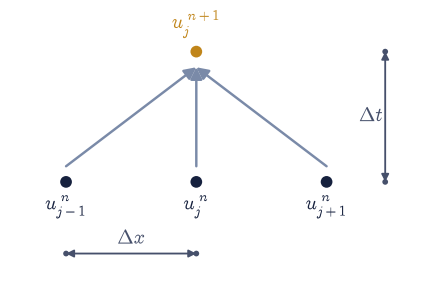
Fig. 71 The FTCS stencil of Eq. 83 on the space–time grid: the new value \(u_j^{n+1}\) at time level \(n+1\) (amber) is assembled from the three values \(u_{j-1}^{n}\), \(u_j^{n}\), \(u_{j+1}^{n}\) at time level \(n\) (ink), with \(\Delta x\) the grid spacing and \(\Delta t\) the time step. Because every value on the right-hand side is already known, the update is explicit; because the new value looks only one cell to each side, the scheme’s domain of dependence per step is exactly \(\pm\Delta x\).#
dx = 0.010, dt = 4.0e-05, C = 0.4, t = 2.0e-03
max |FTCS - exact| = 1.03e-03
peak: FTCS 0.6191 exact 0.6202
integral of u: before 0.12533141 after 0.12533141
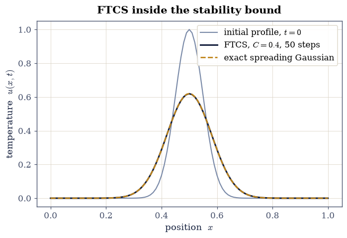
Fig. 72 Explicit FTCS on the diffusion equation \(u_t = Du_{xx}\) with \(D=1\) on the rod \(0\le x\le 1\) with both ends held at \(u=0\): the initial Gaussian hot spot of width \(\sigma_0=0.05\) centred at \(x_0=0.5\) (grey), the numerical profile after \(50\) steps at \(C=0.4\) (ink), and the exact spreading-Gaussian solution Eq. 94 at the same time \(t=2\times10^{-3}\) (amber dashed). The pulse has broadened from \(\sigma_0\) to \(\sqrt{\sigma_0^2+2Dt}\) and its peak has fallen by that same ratio, with the walls not yet involved.#
Validation 2#
✓ FTCS at C = 0.4 reproduces the exact spreading Gaussian [max|Δ| = 0.00103302 (rtol=1e-06, atol=0.002)]
✓ the scheme conserves the integrated heat while the walls stay cold [got 0.125331 vs expected 0.125331 (rtol=1e-06, atol=1e-09)]
True
Exercise 3 — Von Neumann’s amplification factor#
Here is the centrepiece of the notebook. A marching scheme is a linear map, so ask what it does to a single Fourier mode and the whole stability question collapses to one number. Substituting \(u_j^{\,n} = A^n e^{\mathrm i\theta j}\) into Eq. 83 gives the amplification factor Eq. 84, \(A(\theta) = 1 - 4C\sin^2(\theta/2)\), and stability is the statement that no representable mode grows, \(|A(\theta)| \le 1\) for all \(|\theta| \le \pi\).
On this grid the analysis is not merely suggestive, it is exact, and that is worth dwelling on. With both ends held at zero, the sampled sine \(\sin(m\pi x_j/L)\) is an exact eigenvector of the three-point second difference: \(\sin[m\pi(x_j\pm\Delta x)/L]\) summed gives \(2\cos(m\pi\Delta x/L)\sin(m\pi x_j/L)\), so
and the boundary values stay exactly zero as the mode evolves. A grid seeded with one such mode is therefore multiplied by exactly \(A(\theta_m)\) per step, so a measured ratio can be compared with the predicted factor to machine precision rather than to a plausible tolerance. On \(101\) points of \([0,1]\) the modes run from \(m=1\) (\(\theta \approx 0.031\), the smoothest) to \(m=99\) (\(\theta \approx 3.11\), one wavelength per two cells: the sawtooth).
Part a) Write amplification_ftcs(C, theta) returning
\(1 - 4C\sin^2(\theta/2)\) from Eq. 84, vectorized over an array of
\(\theta\). Write this one yourself — the analysis is the lesson.
Part b) Evaluate \(|A(\theta)|\) on \(\theta \in [0,\pi]\) for \(C = 0.25\), \(0.5\) and \(0.6\) and plot the three curves against the line \(|A|=1\) (Fig. 73), reading off which \(\theta\) crosses first.
Part c) Measure it. For \(m = 1\), \(20\) and \(99\), seed \(\sin(m\pi x)\) on the
\(101\)-point grid, take exactly one step of the ftcs_diffusion you wrote in
Exercise 2 at \(C = 0.25\) and at \(C = 0.4\), and form the ratio of new to old at the
grid point of largest amplitude. Compare each with \(A(\theta_m)\) from
Eq. 95.
Part d) Impose \(|A| \le 1\) numerically: scan \(C\) over \([0.4, 0.6]\) in steps of \(10^{-4}\), and for each \(C\) take the maximum of \(|A|\) over \(\theta \in [0,\pi]\). The largest \(C\) that survives is the bound Eq. 85, \(C = 1/2\), that is \(\Delta t \le \Delta x^2/2D\).
m = 1 (theta = 0.031), C = 0.25: measured +0.99975328018287 predicted +0.99975328018287
m = 1 (theta = 0.031), C = 0.4: measured +0.99960524829259 predicted +0.99960524829259
m = 20 (theta = 0.628), C = 0.25: measured +0.90450849718747 predicted +0.90450849718747
m = 20 (theta = 0.628), C = 0.4: measured +0.84721359549996 predicted +0.84721359549996
m = 99 (theta = 3.110), C = 0.25: measured +0.00024671981713 predicted +0.00024671981713
m = 99 (theta = 3.110), C = 0.4: measured -0.59960524829259 predicted -0.59960524829259
largest C with max|A| <= 1: 0.5000 (theory: 0.5)
which is dt <= dx^2/(2D) = 5.0e-05 on this grid
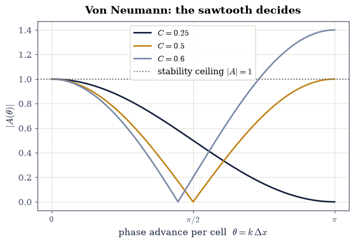
Fig. 73 The FTCS amplification factor Eq. 84, \(|A(\theta)| = |1-4C\sin^2(\theta/2)|\), against the phase advance per cell \(\theta = k\Delta x\) for three diffusion numbers \(C = D\Delta t/\Delta x^2\). At \(C=0.25\) (ink) every mode is damped; at \(C=0.5\) (amber) the sawtooth \(\theta=\pi\) sits exactly on \(|A|=1\) and is merely sign-flipped; at \(C=0.6\) (grey) it exceeds one and grows by \(|1-4C|=1.4\) per step. The shortest representable wavelength is always the first to go unstable, which is why an unstable run erupts at the grid scale.#
Validation 3#
✓ the measured per-step factor of a seeded mode equals 1 - 4C sin^2(theta/2) [max|Δ| = 7.77156e-16 (rtol=1e-06, atol=1e-12)]
✓ imposing |A| <= 1 gives the bound C = 1/2, i.e. dt <= dx^2/(2D) [got 0.5 vs expected 0.5 (rtol=1e-06, atol=0.0002)]
True
Exercise 4 — Just inside the bound, and just outside it#
A bound is only convincing when the run on the wrong side of it actually fails, so we take the same hot-spot problem of Exercise 2 and march it twice: once at \(C = 0.48\) and once at \(C = 0.52\), a difference of eight percent in the time step and nothing else. Both runs go to the same physical time \(t = 0.04\), which takes \(833\) steps at \(C=0.48\) (\(\Delta t = 4.8\times10^{-5}\)) and \(769\) steps at \(C = 0.52\) (\(\Delta t = 5.2\times10^{-5}\)). By Eq. 84 the second run amplifies the sawtooth by \(|1-4C| = 1.08\) per step while flipping its sign.
One feature of the unstable run is worth predicting before seeing it, because it is the reason unstable code so often ships. The initial Gaussian is smooth, so its sawtooth content is not merely small, it is at the level of the floating-point dust of §0.1, around \(10^{-16}\). Growing that to something visible at \(1.08\) per step takes roughly \(\ln(10^{16})/\ln(1.08) \approx 480\) steps. An unstable run therefore looks perfectly healthy for hundreds of steps and then erupts, seemingly without cause. Nothing changed at the moment of eruption: the exponential was there from the first step, feeding on round-off.
Part a) March the Exercise 2 initial profile with your ftcs_diffusion at
\(C = 0.48\) for \(833\) steps and report \(\max_j|u_j|\) at the end.
Part b) March the same profile at \(C = 0.52\) for \(769\) steps and report \(\max_j|u_j|\) at the end.
Part c) Measure the growth rate of the unstable run late in the march, when the sawtooth dominates: take \((\max_j|u_j|\) at the final step \(/\max_j|u_j|\) thirty steps earlier\()^{1/30}\) and compare it with the predicted \(|1-4C| = 1.08\).
Part d) Plot the two final profiles on a symmetric-log axis, and the history of \(\max_j|u_j|\) against time for both runs (Fig. 74).
C = 0.48: dt = 4.80e-05, 833 steps to t = 0.04, final max|u| = 1.733e-01
C = 0.52: dt = 5.20e-05, 769 steps to t = 0.04, final max|u| = 3.090e+08
late growth per step at C = 0.52: measured 1.0791 predicted |1-4C| = 1.0800
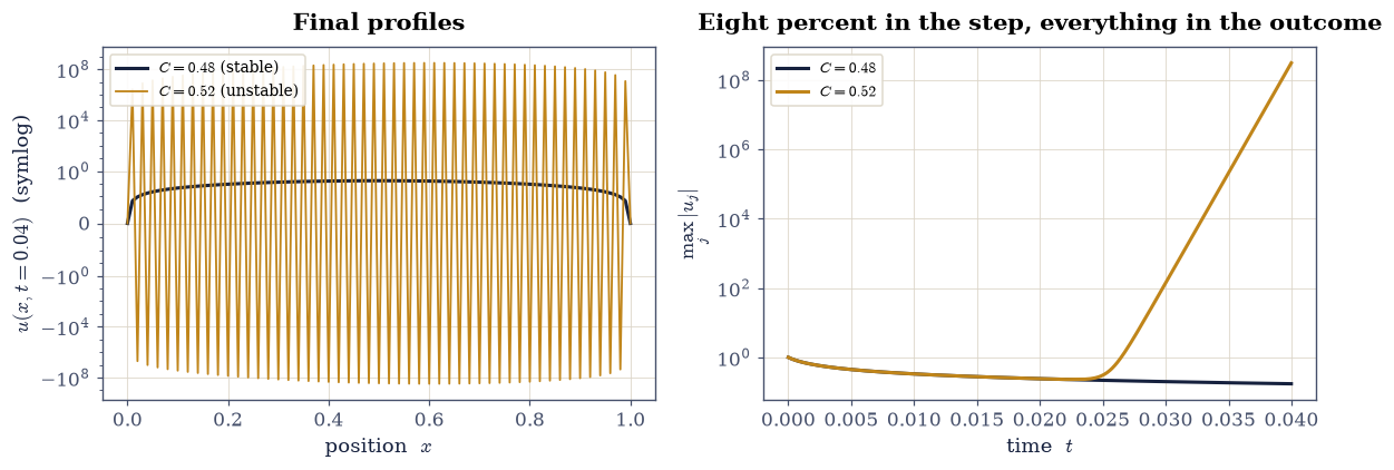
Fig. 74 The stability bound Eq. 85 demonstrated on the diffusion equation with the same initial Gaussian, the same grid (\(\Delta x = 0.01\)) and the same end time \(t=0.04\), differing only in the diffusion number \(C = D\Delta t/\Delta x^2\). Left: the final profiles on a symmetric-log axis, with \(C=0.48\) (ink) a smooth decayed pulse and \(C=0.52\) (amber) a grid-scale sawtooth of amplitude \(\sim 10^{8}\). Right: the history of \(\max_j|u_j|\), falling smoothly inside the bound and rising as \(|1-4C|^n = 1.08^n\) outside it, after a quiet interval in which the unstable mode climbs out of the \(10^{-16}\) round-off floor.#
Validation 4#
✓ FTCS is stable at C = 0.48 and explodes at C = 0.52, the only difference being dt [final max|u|: 1.73e-01 vs 3.09e+08]
✓ the unstable run grows at the rate |1 - 4C| that von Neumann predicts [got 1.0791 vs expected 1.08 (rtol=0.02, atol=1e-09)]
True
Exercise 5 — Relaxation is diffusion at the stability limit#
The elliptic case has been solved already, and this exercise is about seeing that it was solved with the machinery of this notebook. §3.4 attacks Laplace’s equation by Jacobi relaxation, Eq. 208: replace every interior value by the average of its neighbours and repeat. Now set \(C = 1/2\) in the explicit diffusion step Eq. 83 and watch the arithmetic: \(u_j + \tfrac12(u_{j+1} - 2u_j + u_{j-1}) = \tfrac12(u_{j+1} + u_{j-1})\). The \(u_j\) term cancels identically, and the explicit diffusion step is the Jacobi sweep, taken at exactly the largest step Eq. 85 allows. Relaxation is not merely analogous to letting heat settle down; it is the same code, and marching the parabolic problem to steady state solves the elliptic one, because \(\partial_t u \to 0\) is \(u_{xx} = 0\).
The correspondence extends to the convergence rate. Jacobi’s error falls by the spectral radius \(\rho(M)\) per sweep, Eq. 211, and von Neumann has already computed that number for us: at \(C = 1/2\) the amplification factor Eq. 84 is \(A = 1 - 2\sin^2(\theta/2) = \cos\theta\), whose largest magnitude over the modes that survive the boundary conditions belongs to the smoothest one, \(\theta_1 = \pi\Delta x/L\). So \(\rho = \cos(\pi\Delta x/L)\), which for a fine grid is \(1 - O(\Delta x^2)\): agonizingly close to one, which is exactly why §3.4 needs Gauss–Seidel and SOR. The slow mode of relaxation and the slow mode of diffusion are the same physics.
The test problem is the simplest elliptic one there is: \(u_{xx} = 0\) on \([0,1]\) with \(u(0)=0\) and \(u(1)=1\), sampled on \(41\) points (\(\Delta x = 0.025\)), started from \(u=0\) everywhere in the interior. Its exact solution is the straight line \(u(x) = x\), the 1-D harmonic function, and there is nothing else it could be: a harmonic function has no interior extremum, so it cannot bulge either way.
Part a) Take one step of your ftcs_diffusion at \(C = 0.5\), and independently
form the neighbour average \(\tfrac12(u_{j+1} + u_{j-1})\) on the interior with a
slice expression. Do it twice: once from the initial state above, and once from a
generic bumpy profile with nothing special about it. Confirm the two arrays agree.
Do not skip the second profile. Started from \(u=0\) with a single hot boundary, almost every interior node is \(0\) either way and the one that is not comes out exactly \(0.5\) from both expressions — the two agree bit for bit, but only because the arithmetic never had to round. That would be a check that cannot fail, and a check that cannot fail measures nothing. On a generic profile the cancellation is still an exact identity in real arithmetic, but the two expressions round it differently: \(u_j + \tfrac12(u_{j+1} - 2u_j + u_{j-1})\) performs three additions where \(\tfrac12(u_{j+1} + u_{j-1})\) performs one, so expect them to part company in the last bit and nowhere above it. That gap is §0.1’s subject, not a flaw in the identity.
Part b) March \(4000\) steps at \(C = 0.5\) and compare the result with \(u(x) = x\), reporting \(\max_j|u_j - x_j|\).
Part c) Measure the asymptotic convergence rate: with \(e_k = \max_j|u_j - x_j|\) after sweep \(k\), form \((e_{3000}/e_{2000})^{1/1000}\) and compare it with \(\cos(\pi\Delta x/L)\).
Part d) Plot the profile after \(0\), \(50\), \(200\), \(1000\) and \(4000\) sweeps against the exact straight line (Fig. 75).
from the relaxation start: max |FTCS at C=1/2 - Jacobi sweep| = 0.0e+00
from a generic profile: max |difference| = 1.1e-16 (0.5 eps)
max |u - x| after 4000 sweeps = 2.75e-06
error decay per sweep: measured 0.996917334 predicted cos(pi dx/L) = 0.996917334
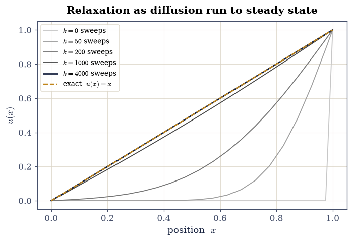
Fig. 75 Jacobi relaxation of the 1-D Laplace problem \(u_{xx}=0\) on \([0,1]\) with \(u(0)=0\), \(u(1)=1\), performed by the explicit diffusion stepper Eq. 83 run at exactly the stability limit \(C=1/2\), where it reduces to the neighbour average Eq. 208. Successive curves (ink, darkening with sweep count \(k\)) show the boundary value diffusing inward from the hot end toward the exact harmonic solution \(u(x)=x\) (amber dashed); the last few percent of the error is carried by the smoothest mode, which decays by only \(\cos(\pi\Delta x/L) = 0.9969\) per sweep.#
Validation 5#
✓ at C = 1/2 the explicit diffusion step IS the Jacobi sweep of section 3.4 [max|Δ| = 1.11022e-16 (rtol=1e-06, atol=1.77636e-15)]
✓ and the comparison is a real one: the two expressions round differently [generic-profile gap = 1.1e-16 (0.5 eps), nonzero, so this check could have failed]
✓ marching the parabolic problem to steady state solves the elliptic one [max|u - x| = 2.75e-06 after 4000 sweeps]
✓ the relaxation rate equals the amplification factor cos(pi dx/L) at C = 1/2 [got 0.996917 vs expected 0.996917 (rtol=0.0001, atol=1e-09)]
True
Exercise 6 — The wave equation and the CFL condition#
The hyperbolic case brings a different bound and a much more dramatic failure. The leapfrog scheme Eq. 87 centres the second difference in time as well as space, which makes it three-level: \(u^{n+1}\) needs both \(u^n\) and \(u^{n-1}\). The first step therefore needs its own formula, and for a string released from rest (\(\partial_t u = 0\) at \(t=0\)) the centred derivative gives \(u^{-1} = u^{1}\), so Eq. 87 collapses to
after which the three-level recurrence runs unchanged. Stability now demands the Courant number \(r = c\,\Delta t/\Delta x\) to satisfy Eq. 88, \(r \le 1\), and past that bound the growth per step is the larger root of \(\xi^2 - 2(1-2r^2)\xi + 1 = 0\) at \(\theta = \pi\), namely \(|\xi| = |1-2r^2| + \sqrt{(1-2r^2)^2 - 1}\), which at \(r = 1.05\) equals \(1.877\). Compare that with the \(1.08\) of the diffusion case: the hyperbolic failure is nearly an order of magnitude faster per step, and a run that violates CFL rarely survives a hundred steps.
Fig. 76 draws the reason, which is geometric rather than algebraic. The scheme reaches one cell to each side per step, so the data it can possibly use lies within \(\pm\Delta x\); the true solution at that point is determined by the data within \(\pm c\,\Delta t\), along the characteristics \(x \pm ct\). Stability is the requirement that the second interval fit inside the first, which is Eq. 88 exactly.
The test problem is a string of unit length with clamped ends, wave speed \(c = 1\), sampled on \(401\) points (\(\Delta x = 0.0025\)), plucked into the Gaussian \(u(x,0) = \exp[-(x-0.5)^2/2\sigma^2]\) with \(\sigma = 0.04\) and released from rest. Before the halves reach the walls, d’Alembert’s solution is exact:
so the plucked shape splits into two half-amplitude copies travelling in opposite directions.
Part a) Write leapfrog_wave(u_init, r, n_steps): take the first step with
Eq. 96, then march Eq. 87, holding both end values
at zero throughout, and return the final profile together with the history array of
shape (n_steps + 1, len(u_init)). Write this one yourself — the
implementation is the lesson.
Part b) Run it at \(r = 0.9\) (so \(\Delta t = r\Delta x/c = 2.25\times10^{-3}\)) for \(89\) steps, reaching \(t \approx 0.2\), and compare the result with Eq. 97 point by point.
Part c) Run it at \(r = 1.05\) (\(\Delta t = 2.625\times10^{-3}\)) for \(76\) steps, the same physical time, and report \(\max_j|u_j|\).
Part d) Measure the late growth rate of the unstable run over its final \(20\) steps, as in Exercise 4, and compare it with the predicted \(|\xi| = 1.877\).
Part e) Animate both runs out to \(t = 0.6\), long enough for the stable pulse to reflect off the walls (Fig. 77). Plot the unstable run normalized by its own running maximum, with that maximum reported in the panel title, so that the shape of the instability and the size of it are both visible.

Fig. 76 The Courant–Friedrichs–Lewy condition Eq. 88 as a statement about domains of dependence, drawn in the space–time plane with horizontal distances in units of the grid spacing \(\Delta x\) and the vertical extent one time step \(\Delta t\). In both panels the ink lines bound the numerical domain of dependence of the updated value \(u_j^{n+1}\), which reaches exactly one cell to each side, and the amber lines are the physical characteristics \(x \pm ct\) that determine the true solution there. Left, \(r = c\Delta t/\Delta x = 0.6\): the physical cone lies inside the numerical one and the scheme sees everything it needs. Right, \(r = 1.4\): the physical cone escapes the numerical one, so the scheme is computing an answer that depends on data it never read.#
r = 0.9: dt = 2.250e-03, 89 steps to t = 0.200, max|u| = 5.000e-01
r = 1.05: dt = 2.625e-03, 76 steps to t = 0.200, max|u| = 7.346e+04
stable run vs d'Alembert: max difference = 1.07e-04
late growth per step at r = 1.05: measured 1.8111 predicted |xi| = 1.8773
Fig. 77 Animation of the plucked string \(u_{tt}=c^2u_{xx}\) with \(c=1\), clamped at both ends, marched with the leapfrog scheme Eq. 87 out to \(t=0.6\) on \(401\) grid points. Top, Courant number \(r = c\Delta t/\Delta x = 0.9\): the initial Gaussian splits into two half-amplitude copies that travel outward at speed \(c\), reflect off the clamped ends with inverted sign, and pass back through each other, exactly as d’Alembert’s solution Eq. 97 requires. Bottom, \(r = 1.05\): the same initial data, normalized by the running maximum \(\max_j|u_j|\) printed above the panel, so that the grid-scale sawtooth erupting out of the round-off floor is visible in shape while its amplitude climbs past \(10^{40}\).#
Validation 6#
✓ leapfrog at r = 0.9 reproduces d'Alembert's two counter-propagating halves [max|Δ| = 0.000106946 (rtol=1e-06, atol=0.005)]
✓ leapfrog at r = 1.05 violates CFL and destroys itself in under a hundred steps [max|u| = 7.35e+04 after 76 steps]
✓ the CFL-violating run grows at the rate the amplification quadratic predicts [got 1.81112 vs expected 1.87733 (rtol=0.08, atol=1e-09)]
True
Exercise 7 — Backward Euler: no step ceiling at all#
The cure for a stiff ODE system was to evaluate the right-hand side at the end of the step (Eq. 48), and nothing about that argument cared whether the system came from a chemical network or from a grid. Applying it here gives the implicit scheme Eq. 89, whose amplification factor Eq. 90 is \(1/(1+4C\sin^2(\theta/2))\): a positive number strictly below \(1\) for every \(C>0\), so no step size can make any mode grow. The price is that the unknowns at level \(n+1\) are coupled, so each step is a linear solve rather than an update.
The system is tridiagonal, which makes the price small. Writing the interior
unknowns as a vector, Eq. 89 reads \(M\mathbf u^{n+1} = \mathbf u^{n} +
\mathbf g\), with \(M\) carrying \(1+2C\) on its diagonal and \(-C\) on both off-diagonals,
and \(\mathbf g\) holding \(C\) times the (fixed) boundary values in its first and last
slots. scipy.linalg.solve_banded solves such a system in \(O(n)\) work given the
matrix in banded storage: an array ab of shape (3, n) whose middle row
ab[1, :] is the diagonal, whose top row holds the superdiagonal in ab[0, 1:],
and whose bottom row holds the subdiagonal in ab[2, :-1]. The unused corners stay
zero. Because \(M\) does not change from step to step, it is assembled once outside
the loop. This is the same banded factorization machinery as
§0.4, applied to the narrowest possible band.
The demonstration takes the Exercise 2 hot spot on the same \(101\)-point grid, and marches it at \(C = 25\), that is \(\Delta t = 2.5\times10^{-3}\): fifty times the explicit ceiling Eq. 85 of \(5\times10^{-5}\). Eight such steps reach \(t = 0.02\), by which time the walls matter and the grading reference is the Dirichlet Fourier series of the Setup rather than the free-space Gaussian.
Part a) Write backward_euler_diffusion(u_init, C, n_steps): assemble the
banded array ab described above once, then at each step build the right-hand side
from the interior of \(u^n\) with \(C\,u_0\) added to its first entry and \(C\,u_{N-1}\)
to its last, call scipy.linalg.solve_banded((1, 1), ab, rhs), and write the
result back into the interior. Return the final profile and the history.
Write this one yourself — the implementation is the lesson.
Part b) Run it for \(8\) steps at \(C = 25\) and report \(\max_j|u_j|\), confirming that the peak decreases at every step rather than oscillating.
Part c) Run your explicit ftcs_diffusion at the same \(\Delta t\) for the
same \(8\) steps and report its \(\max_j|u_j|\), for contrast.
Part d) Certify the amplification factor: seed \(\sin(m\pi x)\) for \(m = 1\), \(20\) and \(99\), take one backward-Euler step at \(C = 25\), and compare the measured ratio with Eq. 90.
Part e) Plot the backward-Euler profile at \(t = 0.02\) against the continuum series solution, with the explicit run at the same step on a symmetric-log axis beside it (Fig. 78).
C = 25.0: dt = 2.5e-03, explicit ceiling dx^2/2D = 5.0e-05
backward Euler after 8 steps: max|u| = 0.2531
peak decreasing at every step: True
vs the continuum series: max difference = 1.06e-02
explicit FTCS at the same dt: max|u| = 7.204e+05
m = 1: measured 0.97592206857050 predicted 0.97592206857050
m = 20: measured 0.09479436479137 predicted 0.09479436479137
m = 99: measured 0.00990340927458 predicted 0.00990340927458
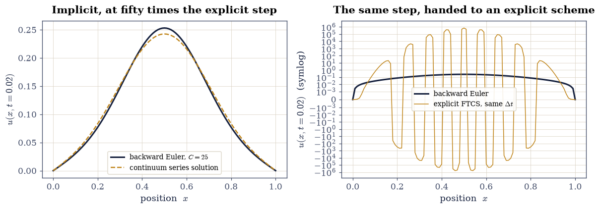
Fig. 78 Backward Euler at a step fifty times the explicit ceiling. Both panels march the Exercise 2 hot spot on the same \(101\)-point grid with \(\Delta t = 2.5\times10^{-3}\) (\(C = D\Delta t/\Delta x^2 = 25\)) for eight steps to \(t=0.02\). Left: the implicit profile (ink) against the continuum Fourier-series solution of the same problem (amber dashed), agreeing to a few percent of the peak. Right, on a symmetric-log axis: the explicit FTCS scheme handed the identical step size (amber) has reached \(\sim 10^{6}\) and is pure grid-scale sawtooth, while the implicit result (ink) is the same smooth curve as on the left. Unconditional stability is the whole difference.#
Validation 7#
✓ backward Euler is stable and monotone at C = 25, fifty times the explicit ceiling [max|u| = 0.253, explicit FTCS at the same dt reached 7.2e+05]
✓ the measured implicit factor equals 1/(1 + 4C sin^2(theta/2)) for every mode [max|Δ| = 5.41234e-16 (rtol=1e-06, atol=1e-12)]
✓ the implicit profile at t = 0.02 matches the continuum series solution [max|Δ| = 0.0105679 (rtol=1e-06, atol=0.02)]
True
Exercise 8 — Crank–Nicolson, and why stability is not accuracy#
Backward Euler is unconditionally stable and only first order in time, which is a poor bargain when a large step is being taken precisely because it is affordable. Averaging the spatial operator between the two time levels, the trapezoid rule in time, gives Crank–Nicolson Eq. 91: still one tridiagonal solve per step, now with \(1+C\) on the diagonal and \(-C/2\) off it, but second order in \(\Delta t\), and with the amplification factor Eq. 92 still bounded by one for every \(C\).
Measuring that second order takes some care, because a run carries two independent errors and we want only one of them. The trick is to grade against the exact solution of the semi-discrete problem, the ODE system the grid actually solves, rather than the continuum PDE. By Eq. 95 the sampled sines are exact eigenvectors of the discrete Laplacian, so if the initial data is a combination of them the semi-discrete solution is available in closed form. Taking \(u(x,0) = \sin(\pi x) + \tfrac12\sin(7\pi x)\) on the \(101\)-point grid,
which contains no spatial discretization error at all: whatever remains when a scheme is compared with it is purely the error of its time stepping.
The exercise closes with the caveat that gives this notebook its shape. At \(C = 25\), Eq. 92 gives \(A_{\text{CN}}(\pi) \approx -0.96\), so Crank–Nicolson keeps the sawtooth almost undamped and merely flips its sign each step, whereas backward Euler’s Eq. 90 crushes it to \(0.0099\). Both are unconditionally stable. Only one of them is a good idea for data with sharp features at a large step, and no stability analysis will ever tell us that: stability says nothing grows, not that anything is right. This is also why §8.16 can lean on Crank–Nicolson for the time-dependent Schrödinger equation, where \(|A| = 1\) exactly is not a defect but the requirement, unitarity.
Part a) Write crank_nicolson_diffusion(u_init, C, n_steps), following the
pattern of Exercise 7 but with the banded matrix carrying \(1+C\) on the diagonal and
\(-C/2\) on both off-diagonals, and with the right-hand side
\(u^n + \tfrac{C}{2}\delta^2 u^n\) (plus \(\tfrac{C}{2}\) times the boundary values in
its end slots).
Part b) Confirm it is unconditionally stable too: run the Exercise 2 hot spot for \(8\) steps at \(C = 25\) and report \(\max_j|u_j|\).
Part c) Measure the order in time. With \(u(x,0)=\sin(\pi x)+\tfrac12\sin(7\pi
x)\) and \(T = 0.01\), run both implicit schemes with \(n = 8, 16, 32, 64, 128, 256\)
steps, take the maximum error against Eq. 98, and fit the slopes
with the Setup’s fit_order. Backward Euler should give \(1\) and Crank–Nicolson
\(2\) (Fig. 79).
Part d) Evaluate both amplification factors at \(\theta = \pi\) and \(C = 25\) and state what each does to a sawtooth.
Crank-Nicolson at C = 25.0: max|u| = 0.2424
fitted order in time: backward Euler 1.06, Crank-Nicolson 2.00
at C = 25.0, sawtooth factor: backward Euler +0.0099 (crushed), Crank-Nicolson -0.9608 (sign-flipped, barely damped)
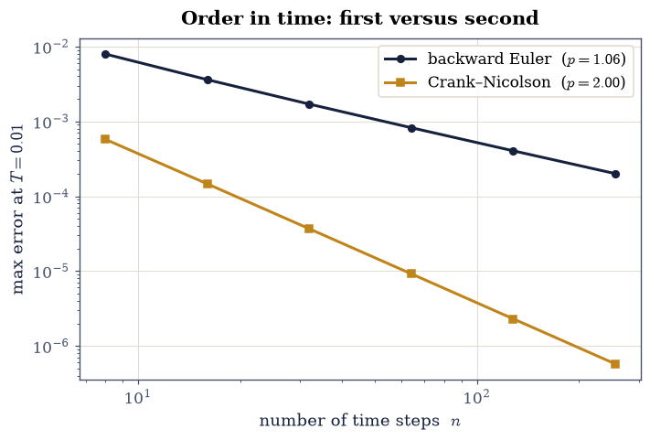
Fig. 79 Temporal convergence of the two implicit schemes on the diffusion equation, graded against the semi-discrete exact solution Eq. 98 so that no spatial error contaminates the measurement. The initial data is \(\sin(\pi x)+\tfrac12\sin(7\pi x)\) on \(101\) grid points, marched to \(T=0.01\) with \(n\) steps: backward Euler (ink) falls with slope \(-1\) and Crank–Nicolson (amber) with slope \(-2\), the fitted orders shown in the legend. Both are unconditionally stable, so the only question left between them is accuracy.#
Validation 8#
✓ Crank-Nicolson is stable at C = 25 as well [max|u| = 0.2424]
✓ backward Euler is first order in time [got 1.05935 vs expected 1 (rtol=1e-06, atol=0.15)]
✓ Crank-Nicolson is second order in time [got 1.99539 vs expected 2 (rtol=1e-06, atol=0.1)]
✓ stability is not accuracy: at C = 25 Crank-Nicolson leaves the sawtooth almost undamped while backward Euler crushes it [A(pi): Crank-Nicolson -0.9608, backward Euler 0.0099]
True
Exercise 9 — The spectral alternative, and choosing a scheme#
Everything so far has been a contest between finite-difference schemes, but on a periodic domain there is an option that leaves the contest entirely. Fourier modes are exact eigenfunctions of \(\partial_x^2\), so on a ring the diffusion equation uncouples into one scalar ODE per wavenumber with the closed-form solution Eq. 93, \(\hat u(k,t) = \hat u(k,0)e^{-Dk^2t}\). There is no time step to choose, no stability condition to respect, and no truncation error in time: a single multiplication in Fourier space carries the solution to any \(t\) we like. The spatial derivative is exact too, up to the mode truncation, rather than \(O(\Delta x^2)\). This is the same idea as the split-step Fourier propagator of §6.13, which alternates a Fourier half-step for the kinetic operator with a real-space multiplication for the potential, and it is why that notebook never had to think about a step ceiling.
The comparison problem is the diffusion equation on the periodic ring \([0,1)\) with \(D=1\), sampled at \(N=128\) points (\(x_n = n/N\)), with the two-mode initial condition \(u(x,0) = \cos(2\pi x) + \tfrac12\cos(6\pi x)\), whose exact solution is \(e^{-D(2\pi)^2t}\cos(2\pi x) + \tfrac12 e^{-D(6\pi)^2t}\cos(6\pi x)\), run to \(T = 0.01\).
That leaves the practical question the notebook exists to answer, and it now has a short answer. If the problem is elliptic there is no marching to do: relax or factorize (§3.4). If it is parabolic, the explicit scheme is fine whenever \(\Delta t \le \Delta x^2/2D\) is affordable, and since that ceiling falls quadratically with the grid spacing, on a fine grid it usually is not: go implicit, and prefer Crank–Nicolson unless the data has sharp features that need backward Euler’s damping. If it is hyperbolic, explicit marching is the natural choice, because the CFL ceiling \(\Delta t \le \Delta x/c\) falls only linearly and is normally what accuracy wanted anyway. And if the geometry is periodic and the solution smooth, a spectral method beats all of them.
Part a) Take the spectral step: form numpy.fft.rfft of the initial data,
multiply by \(e^{-Dk^2T}\) with \(k = 2\pi\,\)numpy.fft.rfftfreq(N, d=dx), and invert
with numpy.fft.irfft. One operation, no loop.
Part b) Compare the result with the exact two-mode solution above.
Part c) March the same problem with an explicit FTCS update on the periodic
grid, using numpy.roll for the neighbours, at \(C = 0.4\) (that is
\(\Delta t = 2.44\times10^{-5}\)). Report how many steps it takes to reach \(T\) and
how well it does.
Part d) Plot the initial data, the two computed profiles, and the exact solution together (Fig. 80).
spectral: 1 operation, max error = 3.33e-16
FTCS: 410 steps of dt = 2.44e-05, max error = 5.13e-04
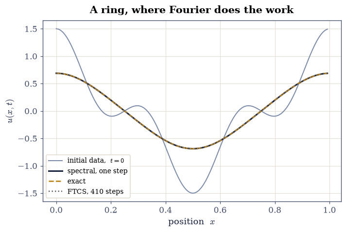
Fig. 80 The spectral propagator against the explicit march on the periodic ring \([0,1)\) with \(N=128\) points, \(D=1\), initial data \(\cos(2\pi x)+\tfrac12\cos(6\pi x)\) (grey), evolved to \(T=0.01\). A single multiplication by \(e^{-Dk^2T}\) in Fourier space Eq. 93 (ink) lands on the exact solution (amber dashed) to \(3\times10^{-16}\), while \(410\) explicit FTCS steps at the largest stable \(\Delta t\) (dotted) arrive with an error near \(5\times10^{-4}\). The short mode has decayed almost completely, the long one by a third.#
Validation 9#
✓ the spectral step is exact in time for the linear diffusion equation [max|Δ| = 3.33067e-16 (rtol=1e-06, atol=1e-12)]
✓ 410 explicit steps at the stability limit reach the same answer, less precisely [max|Δ| = 0.000512543 (rtol=1e-06, atol=0.002)]
True
With your assistant
Ask your assistant for the 2-D explicit diffusion stepper on a square grid, the
natural sequel to the 1-D ftcs_diffusion above. Then run the von Neumann
argument on what it returns: substitute \(A^n e^{\mathrm i(\theta_x j + \theta_y l)}\)
into its update, and check whether the stability bound it inherits is the 1-D
\(\Delta t \le \Delta x^2/2D\) or the stricter \(\Delta t \le \Delta x^2/4D\) that two
dimensions demand. Confirm your answer by running the thing on either side of the
bound. The check is yours.
Notebook summary#
The discriminant of Eq. 80 sorts second-order PDEs into elliptic, parabolic and hyperbolic, and the sort decides the method: elliptic problems have no marching direction and are relaxed or factorized (§3.4), while parabolic and hyperbolic ones are marched, at a step that is not freely ours.
Discretizing space turns a PDE into a stiff ODE system whose stiffness grows as \(4D/\Delta x^2\), so §0.7’s bound \(h\le 2/k\) already predicts the explicit ceiling. Von Neumann’s amplification factor \(A = 1-4C\sin^2(\theta/2)\) Eq. 84 reproduces it exactly, and we measured \(A\) against the formula to \(10^{-12}\) on seeded modes: \(|A|\le1\) requires \(C\le1/2\), that is \(\Delta t \le \Delta x^2/2D\).
The bound bites. On identical grids and to the same \(t=0.04\), \(C=0.48\) ended at \(\max|u|\approx0.17\) and \(C=0.52\) at \(3\times10^{8}\), growing by the predicted \(|1-4C| = 1.08\) per step after climbing out of the \(10^{-16}\) round-off floor (§0.1) for several hundred quiet steps.
At \(C=1/2\) exactly, the explicit diffusion step reduces algebraically to the Jacobi sweep of §3.4 — exactly in real arithmetic, and on a generic profile to within one unit in the last place, the two expression orders rounding differently — and its measured relaxation rate \(0.996917\) per sweep is \(\cos(\pi\Delta x/L)\), the spectral radius that notebook needed SOR to beat.
For the wave equation the leapfrog scheme is stable only under CFL, \(r = c\Delta t/\Delta x \le 1\): at \(r=0.9\) it reproduced d’Alembert’s split pulse to \(10^{-4}\), and at \(r=1.05\) it grew by the predicted \(1.877\) per step and reached \(7\times10^{4}\) within \(76\) steps. The bound is only linear in \(\Delta x\), which is why explicit wave codes remain practical.
Implicit schemes have no ceiling. At \(C=25\), fifty times the explicit limit, both backward Euler Eq. 90 and Crank–Nicolson Eq. 92 stayed bounded where FTCS reached \(7\times10^{5}\); their fitted temporal orders came out \(1.06\) and \(2.00\). Crank–Nicolson’s sawtooth factor at that step is \(-0.96\) against backward Euler’s \(0.0099\): unconditionally stable, and unconditionally stable are not the same as accurate.
On a periodic ring the Fourier modes diagonalize the problem, and one multiplication by \(e^{-Dk^2T}\) Eq. 93 matched the exact solution to \(3\times10^{-16}\) where \(410\) explicit steps managed \(5\times10^{-4}\).
Outlook#
Two and three dimensions tighten the explicit bound to \(\Delta t \le \Delta x^2/(2d\,D)\) in \(d\) dimensions, and make the implicit solve a sparse system rather than a tridiagonal one. The classical escape is operator splitting: alternating-direction implicit (ADI) schemes solve one tridiagonal system per axis per step and keep both the unconditional stability and the \(O(n)\) cost.
Nonlinear and advective problems break the analysis, since von Neumann assumes constant coefficients. Freezing the coefficients locally is the working compromise, and for advection the centred stencil is not merely restricted but unconditionally unstable, which is what motivates upwind and flux-limited schemes.
Beyond finite differences lie finite elements (unstructured geometry) and full spectral methods (exponential accuracy on smooth periodic problems), the latter already at work in §6.13.
Stability with structure. Crank–Nicolson conserves the norm of a Schrödinger wave function exactly rather than approximately, which is the PDE analogue of the symplectic-integrator lesson from §1.6: a scheme that respects the equation’s structure outperforms a scheme that merely has a higher order. §8.16 is that argument in production.
References#
William H. Press, Saul A. Teukolsky, William T. Vetterling, and Brian P. Flannery. Numerical Recipes: The Art of Scientific Computing. Cambridge University Press, 3 edition, 2007.