1.3 The Double Pendulum

Elementary Computational Physics

Volume I — Elementary Mechanics Notebook 1.3

From a two-line Lagrangian to deterministic chaos: equations of motion, energy conservation, the phase portrait, sensitive dependence, and a kernel-free animation.

Level · intermediate   •   Est. · 60–90 min

Raymond Amador v1.4.0  ·  2026-07-31  ·  CC BY 4.0 (text) / MIT (code)

Notebook overview

The double pendulum (a pendulum hung from the end of another pendulum) is the smallest mechanical system most students meet that is genuinely chaotic. It is fully deterministic: given the initial angles and angular velocities, Newton (or, more comfortably, Lagrange) fixes the entire future. Yet two starts that differ by a hair diverge exponentially, so in practice the motion is unpredictable. That tension (determinism without predictability) is the whole pedagogical point, and it is best seen rather than described, which is exactly what a notebook is good for.

We will (1) set up coordinates and the Lagrangian, (2) obtain the equations of motion (once by hand, once symbolically with SymPy as a check), (3) integrate them numerically, (4) verify the solution by watching the total energy stay constant, (5) draw the phase portrait, (6) measure sensitive dependence on initial conditions, and (7) animate the motion.

Scope. This is a working review, not a textbook chapter. For the analytical mechanics behind it, see Nolting, Theoretische Physik 1–2 (Klassische Mechanik) [Nol16a, Nol16b]; Goldstein, Poole & Safko, Classical Mechanics [GPS02]; and, for the geometry of chaos, Strogatz, Nonlinear Dynamics and Chaos [Str15].

Theory in brief

Coordinates and the Lagrangian

Take two point masses \(m_1, m_2\) on massless rigid rods of lengths \(\ell_1, \ell_2\). Measure both angles \(\theta_1, \theta_2\) from the downward vertical. The bob positions are

\[ x_1 = \ell_1 \sin\theta_1, \quad y_1 = -\ell_1 \cos\theta_1, \qquad x_2 = x_1 + \ell_2 \sin\theta_2, \quad y_2 = y_1 - \ell_2 \cos\theta_2 . \]

Differentiating gives the kinetic energy \(T = \tfrac12 m_1(\dot x_1^2 + \dot y_1^2) + \tfrac12 m_2(\dot x_2^2 + \dot y_2^2)\) and the potential energy \(V = m_1 g y_1 + m_2 g y_2\). The Lagrangian is \(\mathcal{L} = T - V\):

\[ \mathcal{L} = \tfrac12 (m_1+m_2)\ell_1^2\dot\theta_1^2 + \tfrac12 m_2 \ell_2^2 \dot\theta_2^2 + m_2 \ell_1 \ell_2 \dot\theta_1 \dot\theta_2 \cos(\theta_1-\theta_2) + (m_1+m_2) g \ell_1 \cos\theta_1 + m_2 g \ell_2 \cos\theta_2 . \]

Equations of motion

The Euler–Lagrange equations \(\frac{d}{dt}\frac{\partial \mathcal L}{\partial \dot\theta_i} - \frac{\partial \mathcal L}{\partial \theta_i} = 0\) yield two coupled second-order ODEs. Solved for the angular accelerations (writing \(\Delta = \theta_1-\theta_2\) and \(D = 2m_1 + m_2 - m_2\cos 2\Delta\)):

\[ \ddot\theta_1 = \frac{-g(2m_1+m_2)\sin\theta_1 - m_2 g \sin(\theta_1-2\theta_2) - 2\sin\Delta\, m_2(\dot\theta_2^2 \ell_2 + \dot\theta_1^2 \ell_1\cos\Delta)} {\ell_1 D}, \]

\[ \ddot\theta_2 = \frac{2\sin\Delta\,\big(\dot\theta_1^2 \ell_1 (m_1+m_2) + g(m_1+m_2)\cos\theta_1 + \dot\theta_2^2 \ell_2 m_2 \cos\Delta\big)} {\ell_2 D}. \]

We will reproduce these symbolically below rather than trust the algebra.

Small oscillations

For \(|\theta_i| \ll 1\) the system linearises to two coupled harmonic oscillators with two normal modes. For the equal case \(m_1=m_2=m,\ \ell_1=\ell_2=\ell\) the mode frequencies are

\[ \omega_\pm^2 = (2 \pm \sqrt{2})\,\frac{g}{\ell}. \]

(Taylor, Classical Mechanics, Ch. 11, carries the linearisation out in full for exactly this system; the general eigenvalue machinery behind it is the subject of §2.7.)

This is our first independent check: any correct integrator, started at tiny amplitude, must oscillate at these frequencies.

The geometry

Two rods hang from a fixed pivot: the first, of length \(\ell_1\), carries bob \(m_1\) at angle \(\theta_1\) from the downward vertical; the second, length \(\ell_2\), hangs from \(m_1\) and carries \(m_2\) at its own angle \(\theta_2\). Both angles are measured from vertical, so the configuration is the pair \((\theta_1, \theta_2)\). The animation later sets these in motion; the still schematic fixes what the symbols mean.

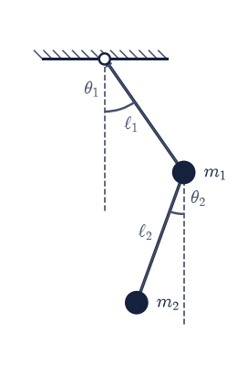
Fig. 87 The double pendulum: a rod of length \(\ell_1\) hangs from the fixed pivot (top) and carries bob \(m_1\) at angle \(\theta_1\) from the downward vertical (dashed); a second rod of length \(\ell_2\) hangs from \(m_1\) and carries bob \(m_2\) at angle \(\theta_2\), measured from the vertical through \(m_1\). The configuration is the angle pair \((\theta_1,\theta_2)\).

---

Setup

Data only: the libraries, and the five numbers that fix the physical system — gravity \(g\), the two bob masses, and the two rod lengths, taken equal unless an exercise says otherwise. Not one function is defined here. Everything this notebook is about — the equations of motion, the integrator wrapper that drives them, the energy meter that certifies the integration, the spectrum that locates the normal modes, the Lyapunov fit, and the animation callback — you write in the exercise where it belongs.

The Setup below holds this notebook’s data and instruments — nothing you are asked to build. It is collapsed so the building stays yours; expand it whenever you want the details.

Show code cell source

Hide code cell source

import numpy as np
from scipy.integrate import solve_ivp
import matplotlib.pyplot as plt

from ecp import validate
from ecp.animate import show


# data: physical parameters (SI). Equal masses and lengths unless stated
# otherwise.
G = 9.81
M1 = M2 = 1.0
L1 = L2 = 1.0

Exercise 1 — Implement the equations of motion

Every later exercise rests on the right-hand side of the ODE system, so the notebook’s first build is also its most consequential. The state it advances is the pair of angles together with their rates, \(\mathbf{y} = (\theta_1, \dot\theta_1, \theta_2, \dot\theta_2)\), and the two angular accelerations obtained above share the denominator \(D = 2m_1 + m_2 - m_2\cos 2\Delta\), which is worth naming once rather than writing twice. Hand algebra of that length is exactly where a sign slips, which is why the check that follows is symbolic rather than numerical: SymPy differentiates the Lagrangian itself, so an error in the hand derivation cannot hide in both routes at once.

1. Write deriv(t, y), returning \((\dot\theta_1, \ddot\theta_1, \dot\theta_2, \ddot\theta_2)\) from the acceleration expressions above. Write this one yourself — the implementation is the lesson.

2. Cross-check it against an independent SymPy derivation from the Lagrangian (the validation below does exactly this at a random state).

Validation 1 — symbolic cross-check of the equations of motion

Rather than trust the hand algebra, derive the accelerations from the Lagrangian with SymPy and confirm they agree with deriv at a random state.

✓  hand-derived EOM match the SymPy derivation   [max|Δ| = 8.88178e-16 (rtol=1e-09, atol=1e-09)]

True

Exercise 2 — Integrate and view the motion

Chaotic systems are unforgiving of sloppy integration: a local error a regular orbit would absorb is amplified exponentially here, so the driver throughout this notebook is scipy.integrate.solve_ivp with DOP853 (an eighth-order explicit Runge–Kutta) at rtol = atol = 1e-10, sampled onto a dense uniform output grid. One trap is worth naming before you fall into it: solve_ivp hands extra arguments to the right-hand side positionally, so a wrapper that forwards a parameter dictionary in whatever order it happens to hold would let a caller who overrides \(m_2\) alone have that value bind silently to \(m_1\) — a physics error with no traceback. Match the parameters to deriv’s signature by name.

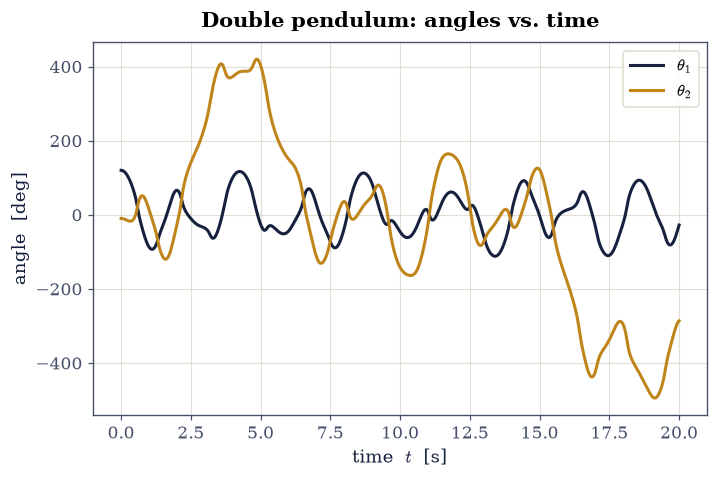
1. Write simulate(y0, t_end, n, **params), integrating the deriv of Exercise 1 under the settings above and returning the solution object.

2. Run it over \(20\) s from the large-amplitude start \((\theta_1, \theta_2) = (120^\circ, -10^\circ)\), released from rest.

3. Plot both angles against time.

Exercise 3 — Total energy as a validation of the integrator

A correct, well-integrated trajectory conserves total mechanical energy — the canonical “did I integrate it right?” check. Neither deriv nor solve_ivp was ever told about energy, so agreement between them is evidence rather than a tautology: \(E = T + V\) is assembled independently from the bob velocities of the Theory section, and whatever drift it shows is accumulated truncation error, not physics.

1. Write total_energy(y), returning \(T + V\) for a state — or, broadcast over the time axis, for a whole state history.

2. Evaluate it along the Exercise 2 trajectory and plot the relative drift \((E - E_0)/|E_0|\) against time.

3. Confirm that drift is tiny.

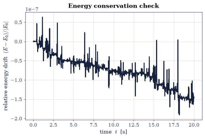
✓  total energy conserved along the trajectory   [max relative drift = 1.90857e-07 (limit 0.0001)]

True

Exercise 4 — Small-amplitude normal modes

At tiny amplitude the system linearises, and its oscillation must sit at a normal-mode frequency \(\omega_\pm^2 = (2\pm\sqrt2)\,g/\ell\) — a check of the physics against linear theory.

1. With the simulate you wrote in Exercise 2, start at small, in-phase angles (which excites mainly the low mode) and integrate a long run.

2. Take the power spectrum of \(\theta_1(t)\) (numpy.fft.rfft/rfftfreq) and locate the dominant peak.

3. Plot the normalised spectrum with both mode frequencies marked.

4. Confirm the peak matches \(\omega_-=\sqrt{(2-\sqrt2)\,g/\ell}\).

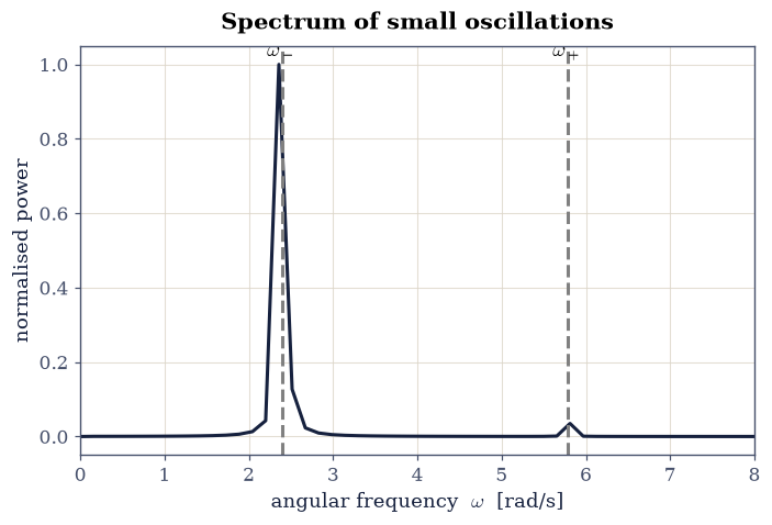
✓  small-amplitude peak matches the low normal mode   [got 2.3559 vs expected 2.3972 (rtol=0.03, atol=1e-09)]

True

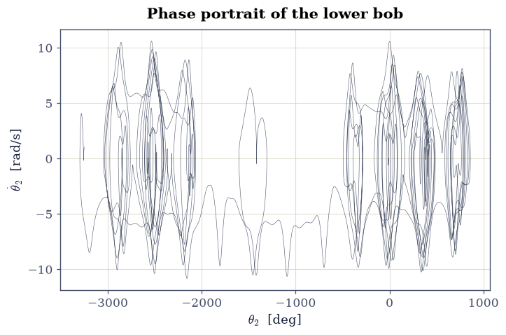
Exercise 5 — Phase portrait

A single pendulum’s phase portrait is a family of closed loops: one degree of freedom, and energy conservation alone already confines the motion to a curve. The double pendulum has two degrees of freedom and still only energy to constrain them, so its trajectory is free to wander a band rather than close — the visual signature of non-integrable motion, and the contrast against every integrable portrait of this volume.

1. With the simulate you wrote in Exercise 2, integrate a long, large-amplitude run (\(120\) s at \(200\) samples per second).

2. Plot the trajectory in the \((\theta_2, \dot\theta_2)\) plane, using a thin, semi-transparent line so that the density shows.

Exercise 6 — Sensitive dependence on initial conditions

Determinism and predictability are not the same thing, and this is where they part company. Two trajectories that start a hair apart separate as \(\delta(t)\sim\delta_0 e^{\lambda t}\) while the separation is still small; the growth rate \(\lambda\) is the largest Lyapunov exponent, and a positive \(\lambda\) is the formal definition of chaos. The exponential law holds only in a window: once \(\delta\) grows to the size of the system itself the two motions are simply unrelated and the curve flattens, so the fit has to be restricted to the growth regime.

1. With the simulate you wrote in Exercise 2, run two trajectories whose initial angles differ by \(\delta_0 = 10^{-6}\) rad and track their separation \(\delta(t)\) in configuration space.

2. Estimate \(\lambda\) from the slope of \(\ln\delta\) over the growth window (numpy.polyfit, before saturation).

3. Plot \(\delta(t)\) on a logarithmic axis together with the fitted exponential.

4. Confirm \(\lambda\) is positive.

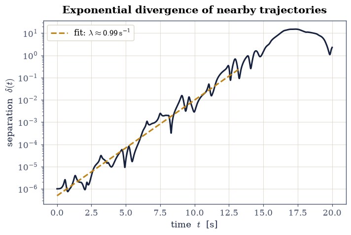
✓  largest Lyapunov exponent is positive (chaotic)   [value = 0.990143]

True

Exercise 7 — Animate the motion

Everything above describes the motion; here you watch it. The rendering path matters as much as the physics: ecp.animate.show pre-renders the frames into a self-contained HTML5 player, so the animation plays on the static course website with no Python kernel behind it.

1. With the simulate you wrote in Exercise 2, integrate a short run (\(12\) s, \(300\) frames) and convert the two angles into bob positions.

2. Build a FuncAnimation of the two rods and the lower-bob trail.

3. Render it with ecp.animate.show.

Once Loop Reflect

Fig. 88 Animation of the double pendulum released from rest at \((\theta_1,\theta_2)=(120^\circ,-10^\circ)\) with equal rods \(\ell_1=\ell_2=1\) and equal bobs \(m_1=m_2=1\): the dark line shows the two rods linking pivot, \(m_1\), and \(m_2\), and the amber curve trails the lower bob \(m_2\).

Notebook summary

• The double pendulum’s equations of motion (matched against a SymPy derivation) integrated with total energy conserved as the integrator check; the small-amplitude normal modes and the phase portrait.

• Sensitive dependence on initial conditions (a positive largest Lyapunov exponent), the signature of deterministic chaos, with the motion animated.

Outlook

• Replace the point bobs with physical rods (moments of inertia) and rederive the Lagrangian. How do the normal-mode frequencies change?

• Build a Poincaré section: record \((\theta_2,\dot\theta_2)\) each time \(\theta_1=0\) with \(\dot\theta_1>0\), and watch regular islands dissolve into a chaotic sea as the energy increases.

• Estimate the Lyapunov exponent properly with the Benettin renormalisation algorithm instead of a single-shot separation fit.

References

[GPS02]

Herbert Goldstein, Charles P. Poole, and John L. Safko. Classical Mechanics. Pearson, 3 edition, 2002.

[Nol16a]

Wolfgang Nolting. Theoretical Physics 1: Classical Mechanics. Springer, 2016. Grundkurs Theoretische Physik 1.

[Nol16b]

Wolfgang Nolting. Theoretical Physics 2: Analytical Mechanics. Springer, 2016.

[Str15]

Steven H. Strogatz. Nonlinear Dynamics and Chaos. Westview Press, 2 edition, 2015.

Take this notebook with you

Use the download button (↓) in the toolbar above to save this notebook and run it yourself. The published notebooks ship without worked solutions; if you would like the reference solutions — to teach from or to check your own work — get in touch: hello@ramador.me.