2.7 Small Oscillations from a General Lagrangian

Elementary Computational Physics

Volume II — Analytical Mechanics Notebook 2.7

Normal modes of any system near equilibrium: linearise the Lagrangian, then simultaneously diagonalise the mass and stiffness matrices — the generalised eigenproblem that underlies molecular vibrations, phonons, and coupled fields.

Level · advanced   •   Est. · 80–100 min

Raymond Amador v1.4.0  ·  2026-07-31  ·  CC BY 4.0 (text) / MIT (code)

Notebook overview

Almost any system, left near a stable equilibrium and nudged gently, rings. A molecule, a bridge, a crystal lattice, a pair of coupled pendula: push them a little and they oscillate, and the motion we see is always a superposition of a few special patterns, the normal modes, each vibrating at its own fixed frequency. This notebook builds the general machine that finds those modes for any Lagrangian system, by linearising the dynamics about equilibrium and solving a single matrix eigenproblem.

This is the culmination of the course’s small-oscillations work, and it ties three earlier threads together. In §1.5 we found the normal modes of a spring chain, but there the masses were uncoupled, so the mass matrix was a multiple of the identity and an ordinary eigenproblem sufficed. Here the kinetic energy couples the coordinates (the mass matrix is genuinely non-diagonal), and the right tool is the generalised eigenproblem \(K\mathbf v = \omega^2 M\mathbf v\). In §1.3 we measured the two natural frequencies of the double pendulum by taking an FFT of a chaotic-looking small-amplitude trajectory; here we derive those same frequencies exactly, in closed form, as eigenvalues. And the symbolic Euler–Lagrange engine from §2.1 does the linearisation for us, straight from the Lagrangian.

How to read the checks. Each exercise ends with a validation that compares our result to an expected physical fact. A ✗ does not by itself mean the answer is wrong: it means the output didn’t match what the check expected, which may be a real error, a different-but-valid convention (a sign, an eigenvector’s overall sign, an array order), or simply too tight a tolerance. Treat a ✗ as a prompt to locate the discrepancy; passing is strong evidence of correctness, not proof.

Scope. This is a working review, not a textbook chapter. For the full theory of small oscillations (the normal-coordinate transformation, the simultaneous diagonalisation theorem, degeneracies from symmetry), see Nolting, Theoretical Physics 2 [Nol16], Goldstein, Poole & Safko, Classical Mechanics [GPS02] ch. 6, and Landau & Lifshitz, Mechanics [LL76] §V.

Theory in brief

Linearising a Lagrangian about equilibrium

Take a system with generalised coordinates \(q_1,\dots,q_n\) and a natural Lagrangian \(\mathcal L = T - V\), where the kinetic energy is quadratic in the velocities. Let \(\mathbf q_0\) be a stable equilibrium: a point where the generalised forces vanish, \(\partial V/\partial q_i|_{\mathbf q_0} = 0\), and \(V\) is a local minimum. Write small displacements \(\eta_i = q_i - q_{0,i}\) and expand to quadratic order.

The kinetic energy becomes a quadratic form in the velocities with the (generally non-diagonal, symmetric, positive-definite) mass matrix

(163)\[T = \tfrac12\,\dot{\boldsymbol\eta}^{\mathsf T} M\, \dot{\boldsymbol\eta}, \qquad M_{ij} = \frac{\partial^2 T}{\partial \dot q_i\,\partial \dot q_j}\bigg|_{\mathbf q_0},\]

and the potential, expanded about the minimum (the constant is irrelevant and the linear term vanishes at equilibrium), becomes a quadratic form with the symmetric stiffness matrix

(164)\[V = \tfrac12\,\boldsymbol\eta^{\mathsf T} K\, \boldsymbol\eta, \qquad K_{ij} = \frac{\partial^2 V}{\partial q_i\,\partial q_j}\bigg|_{\mathbf q_0}.\]

Stability means \(V\) is a genuine minimum, i.e. \(K\) is positive definite.

The equations of motion and the generalised eigenproblem

Feeding the quadratic \(\mathcal L = T - V\) into the Euler–Lagrange equations Eq. 136 gives a linear, coupled system,

(165)\[M\,\ddot{\boldsymbol\eta} = -K\,\boldsymbol\eta.\]

Look for synchronous solutions \(\boldsymbol\eta(t) = \mathbf v\, e^{i\omega t}\), in which every coordinate oscillates with the same frequency \(\omega\) and fixed relative amplitudes \(\mathbf v\). Substituting turns Eq. 165 into the generalised eigenvalue problem

(166)\[K\,\mathbf v = \omega^2\, M\,\mathbf v.\]

The eigenvalues \(\omega_k^2\) are the squared normal-mode frequencies; the eigenvectors \(\mathbf v_k\) are the mode shapes. Because \(M \neq I\) in general, this is not the ordinary eigenproblem \(K\mathbf v = \lambda\mathbf v\) of §1.5: the mass matrix sits on the right-hand side, weighting the eigenproblem. That is the whole generalisation.

Orthogonality and simultaneous diagonalisation

The mode shapes are not orthogonal in the usual sense, but orthogonal with respect to the mass matrix:

(167)\[\mathbf v_i^{\mathsf T} M\, \mathbf v_j = \delta_{ij}, \qquad \mathbf v_i^{\mathsf T} K\, \mathbf v_j = \omega_i^2\,\delta_{ij},\]

where we have normalised each mode so that \(\mathbf v_i^{\mathsf T} M\mathbf v_i = 1\). Collecting the eigenvectors as the columns of a modal matrix \(V = [\mathbf v_1\,\cdots\,\mathbf v_n]\), equation Eq. 167 says \(V^{\mathsf T} M V = I\) and \(V^{\mathsf T} K V = \operatorname{diag}(\omega_k^2)\): the single transformation \(V\) diagonalises both \(M\) and \(K\) at once. In the normal coordinates \(\boldsymbol\xi = V^{\mathsf T} M\,\boldsymbol\eta\) the system decouples completely into \(n\) independent oscillators \(\ddot\xi_k = -\omega_k^2\,\xi_k\): that is the point of the whole construction.

Stability from the spectrum

Because \(M\) is positive definite, the signs of the \(\omega_k^2\) follow the eigenvalues of \(K\). If \(K\) is positive definite every \(\omega_k^2 > 0\) and the system oscillates. If the equilibrium is a saddle, \(K\) has a negative eigenvalue, some \(\omega_k^2 < 0\), and that mode’s \(e^{i\omega t}\) becomes a real exponential \(e^{|\omega| t}\): an instability, not an oscillation. The spectrum diagnoses stability directly.

---

Setup

Data and instruments only: the shared time symbol, the numeric parameter values (equal masses and lengths), the symbolic Euler–Lagrange engine euler_lagrange and the exact double-pendulum Lagrangian — both built from scratch in §2.1 and restated here as tools — plus a symbolic-to-numeric bridge and the bob-geometry helper the animations draw with. This notebook’s own machinery is not here: the linearisation engine linearize, which turns a Lagrangian into the mass and stiffness matrices Eq. 163–Eq. 164, you write in Exercise 1, and the generalised eigenproblem Eq. 166 is solved in the exercises with scipy.linalg.eigh.

The Setup below holds this notebook’s data and instruments — nothing you are asked to build. It is collapsed so the building stays yours; expand it whenever you want the details.

Show code cell source

Hide code cell source

import numpy as np
import sympy as sp
from scipy.integrate import solve_ivp
from scipy.linalg import eigh
import matplotlib.pyplot as plt
from matplotlib.animation import FuncAnimation

from ecp import draw, validate

# built from scratch in §2.1; restated here (via ecp.mechanics) as an instrument.
from ecp.mechanics import euler_lagrange
from ecp.animate import show

t = sp.symbols("t")  # data: the time variable shared by all dynamical coordinates


# built from scratch in §2.1 (Exercise 5, where the bob positions, T and V are
# assembled term by term); restated here as an instrument — the test system this
# notebook's machinery is pointed at, not the machinery itself.
def double_pendulum_lagrangian():
    """The exact equal-mass, equal-length double-pendulum Lagrangian.

    Built symbolically in (θ1, θ2), the test system for the small-oscillation
    machinery.

    Returns
    -------
    tuple
        The Lagrangian and its coordinate symbols.
    """
    m, l, g = sp.symbols("m l g", positive=True)
    th1 = sp.Function("theta1")(t)
    th2 = sp.Function("theta2")(t)
    x1, y1 = l * sp.sin(th1), -l * sp.cos(th1)
    x2, y2 = x1 + l * sp.sin(th2), y1 - l * sp.cos(th2)
    T = sp.Rational(1, 2) * m * (sp.diff(x1, t) ** 2 + sp.diff(y1, t) ** 2)
    T += sp.Rational(1, 2) * m * (sp.diff(x2, t) ** 2 + sp.diff(y2, t) ** 2)
    V = m * g * y1 + m * g * y2
    return T - V, [th1, th2], (m, l, g)


# data: numerical parameter values reused throughout (equal masses and lengths).
M_VAL, L_VAL, G_VAL = 1.0, 1.0, 9.81


# instrument: a symbolic-to-numeric bridge — substituting parameter values and
# casting to float arrays is bookkeeping, not the lesson of any exercise here.
def to_float_matrices(M_sym, K_sym, syms, vals):
    """Substitute numeric parameters and return float NumPy matrices.

    Parameters
    ----------
    M_sym, K_sym : sympy.Matrix
        Symbolic mass and stiffness matrices.
    syms : sequence
        Parameter symbols.
    vals : sequence
        Their numeric values.

    Returns
    -------
    M, K : numpy.ndarray
        The numeric matrices.
    """
    sub = dict(zip(syms, vals))
    M = np.array(M_sym.subs(sub)).astype(float)
    K = np.array(K_sym.subs(sub)).astype(float)
    return M, K


# instrument: drawing geometry — the forward kinematics that turn an angle
# series into bob coordinates for the animations, plumbing rather than physics.
def bob_xy(th1, th2, L=L_VAL):
    """Cartesian positions of the two double-pendulum bobs from the angle series."""
    x1, y1 = L * np.sin(th1), -L * np.cos(th1)
    x2, y2 = x1 + L * np.sin(th2), y1 - L * np.cos(th2)
    return x1, y1, x2, y2

Exercise 1 — From a Lagrangian to \(M\) and \(K\) (the linearisation engine)

Everything downstream rests on extracting the two matrices Eq. 163 and Eq. 164 from a Lagrangian, so the notebook’s first build is also its most consequential. The mass matrix is the Hessian of \(\mathcal L\) in the velocities; the stiffness matrix is minus its Hessian in the coordinates, both evaluated at equilibrium with the velocities set to zero — where, for a natural system with the velocities zeroed, \(\mathcal L = -V\), so that second Hessian is the one of Eq. 164. The natural test system is the small-angle double pendulum of §1.3: its kinetic energy couples \(\dot\theta_1\) and \(\dot\theta_2\), so the mass matrix had better come out non-diagonal.

That test system gives the acceptance test its known answer. With equal masses \(m\) and lengths \(\ell\), and the exact Lagrangian restated in Setup from §2.1, linearising about the hanging equilibrium \(\boldsymbol\theta_0 = (0, 0)\) must give

\[\begin{split} M = m\ell^2\begin{pmatrix} 2 & 1 \\ 1 & 1\end{pmatrix}, \qquad K = mg\ell\begin{pmatrix} 2 & 0 \\ 0 & 1\end{pmatrix}, \end{split}\]

the off-diagonal of \(M\) being the kinematic coupling of the two angles.

1. Write linearize(L, coords, equilibrium), returning the mass and stiffness matrices Eq. 163–Eq. 164 of a Lagrangian about a given equilibrium: substitute zero velocities and the equilibrium coordinates into the two Hessians, \(M_{ij} = \partial^2\mathcal L/\partial\dot q_i\partial\dot q_j\) and \(K_{ij} = -\partial^2\mathcal L/\partial q_i\partial q_j\), and sympy.simplify each entry. Write this one yourself — the implementation is the lesson.

2. Build the exact double-pendulum Lagrangian and run euler_lagrange to see the full (nonlinear) accelerations it implies via Eq. 136.

3. Call your linearize about \(\boldsymbol\theta_0 = (0,0)\) to obtain \(M\) and \(K\), and confirm the mass matrix is non-diagonal and both match the hand-derived matrices above (sympy.simplify on the differences).

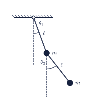
Fig. 151 The equal-mass, equal-length double pendulum near its hanging equilibrium: bobs of mass \(m\) on rods of length \(\ell\) are located by the angles \(\theta_1\) and \(\theta_2\) from the downward vertical (dashed). At small amplitude its kinetic energy couples \(\dot\theta_1\) and \(\dot\theta_2\), making the mass matrix \(M\) non-diagonal.

exact θ̈₁ = (-g*sin(theta1(t) - 2*theta2(t)) - 3*g*sin(theta1(t)) - 2*l*sin(theta1(t) - theta2(t))*Derivative(theta2(t), t)**2 - l*sin(2*theta1(t) - 2*theta2(t))*Derivative(theta1(t), t)**2)/(l*(3 - cos(2*theta1(t) - 2*theta2(t))))

M = [[2*l**2*m, l**2*m], [l**2*m, l**2*m]]
K = [[2*g*l*m, 0], [0, g*l*m]]

✓  the double-pendulum mass matrix is non-diagonal (the coordinates are coupled)   [M[0,1] = l**2*m]
✓  linearise reproduces the hand-derived small-angle M and K

True

Exercise 2 — The generalised eigenproblem → normal frequencies

With \(M\) and \(K\) in hand, the normal-mode frequencies are the eigenvalues of the generalised problem Eq. 166, \(K\mathbf v = \omega^2 M\mathbf v\). Crucially, because \(M\) is not the identity we must solve the generalised problem (passing both \(K\) and \(M\) to scipy.linalg.eigh), not the ordinary eigenproblem of §1.5. For the equal double pendulum the characteristic equation factorises in closed form to

\[ \omega_\pm^2 = (2 \pm \sqrt 2)\,\frac{g}{\ell}, \]

the two frequencies whose beating we extracted by FFT from a small-amplitude trajectory back in §1.3: now obtained exactly as eigenvalues.

Your task. Substitute numbers into \(M\) and \(K\), solve Eq. 166 with eigh(K, M), and confirm the eigenfrequencies \(\omega_k = \sqrt{\omega_k^2}\) equal \(\sqrt{(2 \mp \sqrt 2)\,g/\ell}\).

ω² (eigenvalues) = [ 5.74656495 33.49343505]
ω  (frequencies) = [2.3971994 5.7873513]
ω  (closed form) = [2.3971994 5.7873513]

✓  double-pendulum normal frequencies are √((2∓√2) g/ℓ) (the ω± of §1.3)   [max|Δ| = 1.77636e-15 (rtol=1e-09, atol=1e-09)]

True

Exercise 3 — \(M\)-orthogonality and simultaneous diagonalisation

The mode shapes are orthogonal through the mass matrix, Eq. 167: with the modal matrix \(V\) whose columns are the eigenvectors, \(V^{\mathsf T} M V = I\) and \(V^{\mathsf T} K V = \operatorname{diag}(\omega_k^2)\). The single transformation \(V\) therefore diagonalises both matrices simultaneously: which is exactly why the normal coordinates \(\boldsymbol\xi = V^{\mathsf T} M \boldsymbol\eta\) decouple the dynamics. eigh(K, M) already returns \(M\)-orthonormal eigenvectors, so this is a direct check on the structure.

Your task. Form the matrix products \(V^{\mathsf T} M V\) and \(V^{\mathsf T} K V\) and confirm the first is the identity and the second is diagonal with the \(\omega_k^2\) on its diagonal.

VᵀMV =
 [[ 1. -0.]
 [-0.  1.]]
VᵀKV =
 [[ 5.74656495 -0.        ]
 [-0.         33.49343505]]

✓  the modes are M-orthonormal (VᵀMV = I)   [max|Δ| = 3.33067e-16 (rtol=1e-06, atol=1e-08)]
✓  the modes simultaneously diagonalise K (VᵀKV is diagonal)   [max|Δ| = 3.48173e-15 (rtol=1e-06, atol=1e-08)]

True

Exercise 4 — Mode shapes: in-phase and out-of-phase

Each eigenvector \(\mathbf v_k\) of Eq. 166 is a mode shape: the fixed pattern of relative amplitudes the coordinates hold while oscillating at \(\omega_k\). For the double pendulum the two shapes are physically vivid. The low-frequency mode (\(\omega_-\)) has the two bobs swinging the same way (in phase), so the system is soft and slow; the high-frequency mode (\(\omega_+\)) has them swinging oppositely (out of phase), a stiffer, faster motion. (Only the ratio of the components is physical: an eigenvector’s overall sign is arbitrary.)

Your task. Read the two columns of the eigenvector matrix \(V\) returned by scipy.linalg.eigh, and confirm the low mode has components of the same sign (in phase) while the high mode has components of opposite sign (out of phase).

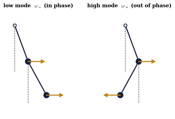
Fig. 152 The two normal-mode shapes of the equal double pendulum, drawn from the eigenvectors \(\mathbf v_\pm\) of Eq. 166. Left: the low-frequency mode \(\omega_-\), with both bobs displaced the same way (in phase). Right: the high-frequency mode \(\omega_+\), with the bobs displaced oppositely (out of phase); amber arrows mark the instantaneous displacement of each bob.

low  mode v = [0.38268343 0.5411961 ],  product of components = +0.207
high mode v = [ 0.92387953 -1.30656296],  product of components = -1.207

✓  mode shapes match the expected patterns: low mode in phase, high mode out of phase   [low product +0.207, high product -1.207]

True

Exercise 5 — A pure mode oscillates at one frequency (worked animation)

The defining property of a normal mode: start the system exactly in one eigenvector and it stays there, every coordinate tracing a sinusoid at the single frequency \(\omega_k\), the shape frozen. We saw this for the uncoupled spring chain in §1.5; here it holds for a genuinely coupled-mass system, and it is the physical content of the simultaneous diagonalisation Eq. 167.

We integrate the linearised equations Eq. 165, \(\ddot{\boldsymbol\eta} = -M^{-1}K\,\boldsymbol\eta\), with scipy.integrate.solve_ivp (DOP853) on a dense t_eval from the initial condition \(\boldsymbol\eta(0) = A\,\mathbf v_-\) (a pure low mode) at rest, and animate the resulting small-amplitude double pendulum. Two independent checks confirm the physics of the integrated data: the energy \(E = \tfrac12\dot{\boldsymbol\eta}^{\mathsf T} M \dot{\boldsymbol\eta} + \tfrac12\boldsymbol\eta^{\mathsf T} K\boldsymbol\eta\) is conserved, and there is no leakage: the projection onto the other mode, \(\xi_{+}(t) = \mathbf v_+^{\mathsf T} M\,\boldsymbol\eta(t)\), stays zero.

This is the worked animation; you build the second in Exercise 6.

energy relative drift = 6.75e-11
max leakage into the other mode = 8.46e-16

Once Loop Reflect

Fig. 153 Animation of the equal double pendulum started purely in its low-frequency normal mode \(\omega_-\) (in-phase) at small amplitude: the whole system oscillates rigidly at the single frequency \(\omega_-=\sqrt{(2-\sqrt2)g/\ell}\), the mode shape held fixed. The amber trail follows the lower bob.

✓  the integrated normal-mode motion conserves energy   [max relative drift = 4.14705e-11 (limit 1e-06)]
✓  a pure normal mode does not excite the other mode (no leakage)   [got 8.46448e-16 vs expected 0 (rtol=1e-06, atol=1e-06)]

True

Exercise 6 — A general motion is a superposition of modes (student animation)

A pure mode is special; a general small-amplitude motion is a superposition of all the modes, each oscillating independently with an amplitude and phase set by the initial conditions. Projecting the initial state onto the modes through the mass matrix gives the modal coefficients \(c_k = \mathbf v_k^{\mathsf T} M\, \boldsymbol\eta_0\) (and \(s_k = \mathbf v_k^{\mathsf T} M\,\dot{\boldsymbol\eta}_0\) for the initial velocities), after which Eq. 167 guarantees the exact closed-form evolution

\[ \boldsymbol\eta(t) = \sum_k \Big(c_k\cos\omega_k t + \tfrac{s_k}{\omega_k}\sin\omega_k t\Big)\,\mathbf v_k . \]

We release the double pendulum from a generic small displacement (only the upper angle displaced) at rest, so both modes are excited.

1. Decompose the initial condition onto the modes, \(c_k = \mathbf v_k^{\mathsf T} M\,\boldsymbol\eta_0\), and reconstruct \(\boldsymbol\eta(t)\) from the sum above.

2. Build the animation: three panels side by side (the full motion and the two modal contributions \(c_k\cos(\omega_k t)\,\mathbf v_k\)), so you can watch the full motion be the sum of its modes. You have the angle time series below; assemble the FuncAnimation, plt.close(fig), then show(...).

3. Confirm the modal superposition reproduces a direct integration of Eq. 165 (scipy.integrate.solve_ivp, DOP853).

A ✗ on the check is about the modal coefficients / reconstruction, not the animation: any correct drawing of the same trajectories is fine. If it fails, inspect the \(c_k = \mathbf v_k^{\mathsf T} M\,\boldsymbol\eta_0\) and the per-mode time evolution.

max |modal − integrated| = 4.05e-12

Once Loop Reflect

Fig. 154 Animation of a generic small-amplitude double-pendulum motion (left) released from the upper angle alone, shown beside its two normal-mode contributions \(c_-\cos(\omega_- t)\,\mathbf v_-\) (centre) and \(c_+\cos(\omega_+ t)\,\mathbf v_+\) (right): the full motion is at every instant the sum of the two modes, with coefficients \(c_k=\mathbf v_k^{\mathsf T} M\boldsymbol\eta_0\) fixed by the initial displacement.

✓  the normal-mode superposition reproduces the directly integrated motion   [max|Δ| = 4.05473e-12 (rtol=1e-06, atol=1e-09)]

True

Exercise 7 — Stability from the spectrum (the contrast)

Everything so far assumed a stable equilibrium, where \(K\) is positive definite and every \(\omega_k^2 > 0\). Now break that. The double pendulum has another equilibrium with the upper bob hanging down but the lower bob balanced straight up, \(\boldsymbol\theta_0 = (0, \pi)\): a saddle of the potential. There the stiffness matrix is indefinite: linearising gives \(K = mg\ell\, \operatorname{diag}(2, -1)\), with one negative eigenvalue. By the stability argument above, that mode has \(\omega^2 < 0\), so its \(e^{i\omega t}\) becomes a real exponential: the inverted bob topples rather than oscillates.

1. Linearise about \(\boldsymbol\theta_0 = (0,\pi)\) with the linearize you wrote in Exercise 1, solve the generalised eigenproblem Eq. 166 with scipy.linalg.eigh(K, M), and confirm one \(\omega^2 < 0\).

2. Integrate Eq. 165 with scipy.integrate.solve_ivp (DOP853) from a tiny displacement and plot the two normal coordinates: one oscillates, the other grows exponentially.

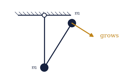
Fig. 155 The saddle equilibrium \(\boldsymbol\theta_0=(0,\pi)\) of the double pendulum: the upper bob \(m\) hangs straight down (\(\theta_1=0\)) while the lower bob is inverted, balanced above its pivot (\(\theta_2=\pi\)), drawn caught mid-topple to show the unstable direction — the amber arrow is the growing perturbation along which the potential falls, so the stiffness matrix \(K\) is indefinite and one normal mode has \(\omega^2<0\).

inverted K = [[2*g*l*m, 0], [0, -g*l*m]]
ω² at the saddle = [-13.87343505  13.87343505]

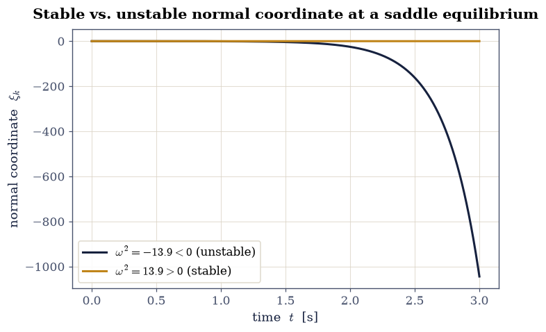
✓  an unstable equilibrium has a negative ω² — a growing mode, not an oscillation   [min ω² = -13.873, |ξ| grew by 35631×]

True

Notebook summary

• The linearisation of a general Lagrangian into mass and stiffness matrices \(M,K\) with the linearize helper built here (packaged for the series as ecp.mechanics.linearize), and the generalised eigenproblem \(K\mathbf v=\omega^2 M\mathbf v\) solved with scipy.linalg.eigh(K, M) (packaged as ecp.mechanics.normal_modes).

• \(M\)-orthonormality of the modes (\(V^\top M V=I\)) and simultaneous diagonalisation; the in-phase and out-of-phase mode shapes; a pure mode oscillating at one frequency; a general motion as a superposition of modes; and stability read from the spectrum.

Outlook

• Molecular vibrations. The longitudinal normal modes of a CO₂-like linear chain of three masses and two springs are a zero-frequency uniform translation and the symmetric and antisymmetric stretches; the translation reflects the chain’s translational symmetry, tying back to the momentum conservation of §2.2. The full three-dimensional molecule adds a doubly-degenerate bending mode, its degeneracy forced by symmetry.

• The continuum limit. Letting the spring chain of §1.5 grow to \(N\to\infty\) turns the discrete normal modes into phonons with a dispersion relation: the same generalised eigenproblem, now the harmonic theory of solids.

• Damped and driven modes. Adding dissipation and a periodic drive makes each normal coordinate a damped driven oscillator (§1.2), so a multi-DOF system shows a resonance peak at each \(\omega_k\).

• Forward links. This same harmonic approximation (diagonalising the Hessian of a potential) is the basis of normal-mode analysis in molecular dynamics (Volume V) and of field quantisation in terms of modes.

References

[GPS02]

Herbert Goldstein, Charles P. Poole, and John L. Safko. Classical Mechanics. Pearson, 3 edition, 2002.

[LL76]

L. D. Landau and E. M. Lifshitz. Mechanics. Volume 1 of Course of Theoretical Physics. Butterworth–Heinemann, 3 edition, 1976.

[Nol16]

Wolfgang Nolting. Theoretical Physics 2: Analytical Mechanics. Springer, 2016.

Take this notebook with you

Use the download button (↓) in the toolbar above to save this notebook and run it yourself. The published notebooks ship without worked solutions; if you would like the reference solutions — to teach from or to check your own work — get in touch: hello@ramador.me.