0.5 Eigenvalues, Diagonalization, and the SVD

Elementary Computational Physics

Volume 0 — Mathematical & Computational Foundations Notebook 0.5

The spectral theorem, the generalized eigenproblem behind every normal mode, and the singular value decomposition — the master factorization that powers least squares, data compression, and the tensor networks of many-body quantum physics.

Level · advanced   •   Est. · 130–170 min

Raymond Amador v1.4.0  ·  2026-07-31  ·  CC BY 4.0 (text) / MIT (code)

Notebook overview

Eigenvalues we already know as the invariant directions of a linear map; what we have probably not seen is how a computer finds them, and that it does so without ever touching the characteristic polynomial, whose roots are far too ill-conditioned to trust (a direct callback to the conditioning lessons of §0.1 and §0.4). This notebook builds the numerical eigenproblem from the well-behaved symmetric case and the spectral theorem, through the QR algorithm that scipy.linalg.eigh actually runs, to the generalized eigenproblem \(K\mathbf v=\lambda M\mathbf v\) that is the literal engine of every normal-mode calculation in §1.5, §2.6, and §2.7.

Size then changes the question. A matrix small enough to write down can simply be handed to eigh, but the ones a physics computation actually produces are huge and almost entirely zeros, and it is the zeros, not the arithmetic, that break the calculation first. So the notebook also assembles a sparse finite-difference Laplacian, writes a Lanczos iteration that never sees the matrix except through products \(A\mathbf x\), and derives the shift-invert trick that turns a method biased toward the largest eigenvalues into the standard tool for the smallest. This is the machinery that §3.4 stores a boundary-value problem with, that §3.9 finds waveguide cutoffs with, and that §7.19 and §8.2 find ground states with: they use it, and this is where it is explained.

Its second half is the singular value decomposition: the one factorization that works for any matrix, square or not, and arguably the most useful in all of applied mathematics. We will see its geometry (every linear map is a rotation, a scaling, and another rotation), prove the Eckart–Young theorem (the best low-rank approximation is the truncated SVD), and watch it strip noise from a nearly-low-rank matrix. That last move (keep the few large singular values, discard the small tail) is, almost verbatim, how the tensor networks of many-body quantum physics tame an exponentially large Hilbert space — a connection this course names and motivates but nowhere implements.

Throughout we lean on §0.4: its condition number \(\kappa\), its QR factorization, and its “never invert” rule all return here. The only animation is the SVD’s geometric action, where motion genuinely shows what a still cannot; the spectra and error plots are static.

How to read the checks. Each exercise ends with a validate call against an independent fact: a reconstruction \(A=V\Lambda V^\top\), a known normal-mode frequency, the closed-form spectrum of a discrete Laplacian, an Eckart–Young error equal to \(\sigma_{k+1}\). A ✓ is strong evidence; a ✗ is a prompt to locate the discrepancy, not a verdict.

Scope. A working review, not a course in matrix computations. See Trefethen & Bau, Numerical Linear Algebra [TB97] (the eig and SVD lectures) and Golub & Van Loan [GVL13].

Theory in brief

The eigenproblem, and why not the characteristic polynomial

An eigenpair of a square matrix \(A\) satisfies

(26)\[A\mathbf v = \lambda\mathbf v,\]

so \(\mathbf v\) is a direction the map only stretches, by the factor \(\lambda\). We learned to find \(\lambda\) as the roots of \(\det(A-\lambda I)=0\), but that is precisely what a numerical eigensolver refuses to do: the map from a polynomial’s coefficients to its roots is wildly ill-conditioned (Wilkinson’s classic warning), so forming the characteristic polynomial and rooting it loses most of the digits. Instead, eigenvalues are found by iteration: repeated orthogonal transformations that drive the matrix toward triangular form.

The symmetric case and the spectral theorem

The friendliest (and most physical) case is a real symmetric \(A=A^\top\) (observables, quadratic forms, mass and stiffness matrices). Its eigenvalues are real and its eigenvectors can be chosen orthonormal, so \(A\) diagonalizes as

(27)\[A = V\Lambda V^\top = \sum_i \lambda_i\,\mathbf v_i\mathbf v_i^\top, \qquad V^\top V = I,\]

the spectral theorem: \(A\) is a weighted sum of orthogonal projectors onto its eigendirections. scipy.linalg.eigh returns exactly this \(V\) and \(\Lambda\).

The QR algorithm

How does eigh get there? By the QR algorithm, which reuses the QR factorization of §0.4 in a strikingly simple loop: factor, then multiply the factors back in the opposite order,

(28)\[A_k = Q_k R_k, \qquad A_{k+1} = R_k Q_k,\]

and repeat. Each \(A_{k+1}=Q_k^\top A_k Q_k\) is an orthogonal similarity of \(A\), so the eigenvalues are preserved, and the iterates converge to (block-)triangular form with the eigenvalues marching out onto the diagonal. (Why so simple a loop converges is genuinely subtle; Trefethen & Bau, Numerical Linear Algebra, Lectures 28–29, supply the convergence theory.)

The generalized eigenproblem

Normal modes do not come as \(A\mathbf v=\lambda\mathbf v\) but as

(29)\[K\mathbf v = \lambda M\mathbf v,\]

with a stiffness matrix \(K\) and a mass matrix \(M\ne I\): exactly the form derived in §2.7. It is solved by eigh(K, M), whose eigenvectors are \(M\)-orthonormal; the \(\lambda\) are the squared normal-mode frequencies. This is the engine under §1.5, §2.6, and §2.7.

Sparsity, and what a matrix-vector product already knows

Everything above assumes the matrix fits in memory as a rectangle of numbers. At the sizes physics reaches it does not, and it does not have to: a finite-difference Laplacian, a tight-binding Hamiltonian and a spin chain in the computational basis all couple each row to a handful of neighbours, so all but \(O(N)\) of their \(N^2\) entries are zero. An \(N\times N\) array of doubles costs \(8N^2\) bytes, a gigabyte just past \(N=10^4\), and a dense factorization of it costs \(O(N^3)\) work on top; storing and factoring the zeros is what fails, long before the physics does. Sparse formats (scipy.sparse) keep only the non-zeros, and the eigensolvers built on them (scipy.sparse.linalg.eigsh) ask the operator for one thing only: the product \(A\mathbf x\).

What products alone can reveal is the Krylov subspace generated by a starting vector \(\mathbf b\),

(30)\[\mathcal K_k(A,\mathbf b)=\operatorname{span}\{\mathbf b,\,A\mathbf b,\,A^2\mathbf b,\, \dots,\,A^{k-1}\mathbf b\},\]

reached in \(k-1\) products. Its dimension \(k\) is tiny beside \(N\), yet for symmetric \(A\) the eigenvalues of \(A\) restricted to \(\mathcal K_k\) (the Ritz values) lock onto the extremes of the spectrum long before they resolve anything in the interior. The bias is not a defect but the whole point: a ground-state energy, a lowest cutoff frequency, a slowest relaxation mode all live at an edge of the spectrum, and never in the middle.

The singular value decomposition

Eigenvalues need a square matrix; the SVD needs nothing of the sort. Every \(m\times n\) matrix factors as

(31)\[A = U\Sigma V^\top, \qquad U^\top U = I,\ V^\top V = I,\]

with \(\Sigma\) diagonal holding the singular values \(\sigma_1\ge\sigma_2\ge \cdots\ge 0\). Geometrically every linear map is therefore the same three acts: rotate (\(V^\top\)), scale along axes (\(\Sigma\)), rotate (\(U\)), so a matrix sends the unit sphere to an ellipsoid whose semi-axes are the \(\sigma_i\). The singular values are \(\sigma_i=\sqrt{\lambda_i(A^\top A)}\), tying the SVD back to the symmetric eigenproblem. (That every matrix admits this factorization is a theorem, not an observation; Trefethen & Bau, Numerical Linear Algebra, Lectures 4–5, prove it.)

Low-rank approximation: Eckart–Young

Truncating the SVD to its \(k\) largest singular values gives the provably best rank-\(k\) approximation of \(A\), and the error is exactly the first discarded singular value:

(32)\[\min_{\operatorname{rank}B\le k}\lVert A-B\rVert_2 = \sigma_{k+1}, \qquad B = \sum_{i=1}^{k}\sigma_i\,\mathbf u_i\mathbf v_i^\top.\]

This single fact is the mathematical core of data compression and of the tensor-network methods of many-body quantum physics alike. (Trefethen & Bau, Numerical Linear Algebra, Lecture 5, gives the short proof.)

Setup

Imports and one display setting — this notebook’s Setup defines no functions at all. It holds NumPy, Matplotlib and SymPy, the four scipy.linalg factorizations the notebook leans on (eigh, eigvalsh, qr, svd), the three scipy.sparse constructors and the Krylov eigensolver eigsh that the sparse exercises are measured against them, time.perf_counter for that measurement, the ecp validation and animation helpers, and a four-digit print precision so that spectra and reconstructions read cleanly. Everything the notebook is about — the QR algorithm iterated from scratch, the generalized eigensolve behind the double pendulum’s normal modes, the sparse Laplacian and the Lanczos iteration that hunts its spectrum, the SVD’s three geometric acts, the rank-\(k\) truncations of Eckart–Young, and the noise-stripping of a nearly-low-rank matrix — you build in the exercise where it is earned.

The Setup below holds this notebook’s data and instruments — nothing you are asked to build. It is collapsed so the building stays yours; expand it whenever you want the details.

Show code cell source

Hide code cell source

import time

import numpy as np
import matplotlib.pyplot as plt
import sympy as sp
from scipy.linalg import eigh, svd, qr, eigvalsh
from scipy.sparse import diags, identity, kron
from scipy.sparse.linalg import eigsh

from ecp import validate
from ecp.animate import show

np.set_printoptions(precision=4, suppress=True)

Exercise 1 — The symmetric eigenproblem and the spectral theorem

The cleanest entry point is a real symmetric matrix, where Eq. 27 promises real eigenvalues and orthonormal eigenvectors. Take the explicit matrix

\[\begin{split} A = \begin{bmatrix} 2 & 1 & 0 \\ 1 & 3 & 1 \\ 0 & 1 & 2 \end{bmatrix}, \end{split}\]

which is symmetric, so the spectral theorem applies.

1. Diagonalize it with scipy.linalg.eigh.

2. Verify both halves of Eq. 27: the eigenvectors are orthonormal (\(V^\top V=I\)) and \(A\) is rebuilt as \(V\Lambda V^\top\).

eigenvalues = [1. 2. 4.]
VᵀV =
 [[ 1. -0. -0.]
 [-0.  1. -0.]
 [-0. -0.  1.]]
VΛVᵀ =
 [[ 2.  1. -0.]
 [ 1.  3.  1.]
 [-0.  1.  2.]]

Validation 1

✓  eigenvectors are orthonormal (VᵀV=I)   [max|Δ| = 2.22045e-16 (rtol=1e-06, atol=1e-10)]
✓  A = VΛVᵀ (spectral theorem)   [max|Δ| = 3.10862e-15 (rtol=1e-06, atol=1e-10)]

True

Exercise 2 — Why not the characteristic polynomial

It is worth seeing why numerical eigensolvers avoid the textbook route. For the same matrix \(A=\begin{bmatrix}2&1&0\\1&3&1\\0&1&2\end{bmatrix}\) of Exercise 1, we compare two routes against an exact reference. Because the coefficients-to-roots map is ill-conditioned (the same kind of amplification \(\kappa\) measured in §0.4), the polynomial route loses accuracy even on this benign \(3\times3\).

1. Compute the exact eigenvalues symbolically (sympy.Matrix.eigenvals) as the reference.

2. Compute them numerically with scipy.linalg.eigvalsh (backward-stable).

3. Form the characteristic polynomial’s coefficients (numpy.poly) and root them (numpy.roots); compare both errors against the reference.

error of eigh             = 1.11e-16
error of roots(charpoly)  = 1.78e-15

Validation 2

✓  the QR-based eigensolver beats rooting the characteristic polynomial   [eigh 1.11e-16 < charpoly 1.78e-15]

True

Exercise 3 — The QR algorithm from scratch

To see how eigh actually converges, we implement the unshifted QR algorithm of Eq. 28 using the very QR factorization built in §0.4. Take the explicit symmetric matrix

\[\begin{split} A = \begin{bmatrix} 4 & 1 & 0 \\ 1 & 3 & 1 \\ 0 & 1 & 2 \end{bmatrix}. \end{split}\]

1. Iterate \(A_k=Q_kR_k\), \(A_{k+1}=R_kQ_k\) with scipy.linalg.qr; each step is an orthogonal similarity, so the spectrum is preserved.

2. Track the off-diagonal norm decaying as the diagonal converges to the eigenvalues (Fig. 30).

3. Confirm the converged diagonal matches scipy.linalg.eigvalsh.

QR-algorithm diagonal = [1.2679 3.     4.7321]
eigvalsh              = [1.2679 3.     4.7321]

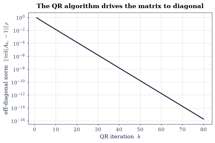
Fig. 30 Convergence of the unshifted QR algorithm Eq. 28 on the symmetric matrix \(A=\bigl[\begin{smallmatrix}4&1&0\\1&3&1\\0&1&2\end{smallmatrix}\bigr]\): the Frobenius norm of the strictly-lower-triangular part (the total off-diagonal magnitude) decays geometrically with iteration on a log axis, as the orthogonal similarities drive \(A_k\) toward the diagonal matrix of its eigenvalues.

Validation 3

✓  the QR algorithm converges to the eigenvalues   [max|Δ| = 4.44089e-15 (rtol=1e-06, atol=1e-06)]

True

Exercise 4 — The generalized eigenproblem (callback to 2.7)

Normal modes arrive as \(K\mathbf v=\lambda M\mathbf v\), Eq. 29, with a mass matrix that is not the identity. Take the small-angle double pendulum of §2.7 with equal bobs and rods (\(m=\ell=1\), \(g=9.81\)), whose mass and stiffness matrices are

\[\begin{split} M = m\ell^2\begin{bmatrix} 2 & 1 \\ 1 & 1 \end{bmatrix}, \qquad K = mg\ell\begin{bmatrix} 2 & 0 \\ 0 & 1 \end{bmatrix}. \end{split}\]

1. Solve the generalized problem with scipy.linalg.eigh(K, M); the eigenvalues are the squared normal-mode frequencies.

2. Confirm they reproduce the analytic doubles \(\omega_\pm^2=(2\mp\sqrt2)\,g/\ell\) — the same modes obtained by direct integration in §1.3 and by linearization in §2.7, here from one eigensolve.

normal-mode frequencies  = [2.3972 5.7874]
analytic √((2∓√2)g/ℓ)    = [2.3972 5.7874]

Validation 4

✓  generalized eig gives the double-pendulum modes √((2∓√2)g/ℓ)   [max|Δ| = 1.77636e-15 (rtol=1e-09, atol=1e-09)]

True

Exercise 5 — Sparse storage: the matrix that is mostly zeros

Every matrix so far has been small enough to write down, and that is the last thing a real physics matrix is. Discretize \(-\nabla^2\) on the unit square with the five-point stencil of §3.4, on an \(n\times n\) grid of interior nodes with Dirichlet boundaries, and the unknowns number \(N=n^2\): a modest \(100\times100\) grid already brings \(N\) to \(10^4\). The operator separates, because the two directions each contribute the same one-dimensional second difference, so it is the Kronecker sum

(33)\[A = D\otimes I_n + I_n\otimes D, \qquad D = \frac{1}{h^2}\operatorname{tridiag}(-1,\,2,\,-1), \qquad h=\frac{1}{n+1},\]

with \(D\) and \(I_n\) of size \(n\times n\) and \(h\) the grid spacing. Each row of \(A\) then carries a diagonal entry and at most four neighbour couplings, so the non-zeros grow like \(5N\) while the dense array that would hold them grows like \(8N^2\) bytes. The scipy.sparse constructors diags, identity and kron assemble Eq. 33 directly in a format that stores only those non-zeros, never the zeros between them.

The assembly can be graded exactly, because this operator’s spectrum is known in closed form: the eigenvectors are the sine products \(\sin(p\pi x)\sin(q\pi y)\) and the discrete eigenvalues are

(34)\[\lambda_{pq} = \frac{4}{h^2}\left[\sin^2\!\frac{p\pi h}{2} + \sin^2\!\frac{q\pi h}{2}\right], \qquad p,q = 1,\dots,n,\]

which reduces to the continuum \(\pi^2(p^2+q^2)\) as \(h\to0\).

1. Write laplacian_2d(n) returning the operator of Eq. 33 in CSR format together with \(h\): build \(D\) with scipy.sparse.diags (values \(-1,2,-1\) on offsets \(-1,0,+1\), scaled by \(1/h^2\)), take the two scipy.sparse.kron products against scipy.sparse.identity(n), add them, and finish with .tocsr(). Call it at \(n=20\) and report A.nnz and the density \(\mathrm{nnz}/N^2\).

2. Certify the assembly: form the dense array with .toarray(), take its spectrum with scipy.linalg.eigvalsh, and compare against Eq. 34 evaluated on the full \((p,q)\) grid.

3. Confirm the structure exactly. An \(n\times n\) grid has \(5n^2-4n\) non-zeros: five per row, less the one missing neighbour for each node on each of the four grid edges.

4. For \(n=10,20,40,80,160,320\) compare the dense cost \(8N^2\) bytes against the bytes CSR actually allocates (A.data.nbytes + A.indices.nbytes + A.indptr.nbytes), and plot both against \(N\) (Fig. 31).

N = 400,  nnz = 1920,  density = nnz/N² = 0.0120
λ_min  numerical    19.7024   analytic    19.7024
λ_max  numerical  3508.2976   analytic  3508.2976
non-zeros 1920 vs 5n²−4n = 1920
    n        N     dense        sparse     ratio
   10      100        0.1 MB    0.006 MB        14×
   20      400        1.3 MB    0.025 MB        52×
   40     1600       20.5 MB    0.100 MB       204×
   80     6400      327.7 MB    0.406 MB       808×
  160    25600     5242.9 MB    1.631 MB      3215×
  320   102400    83886.1 MB    6.538 MB     12830×

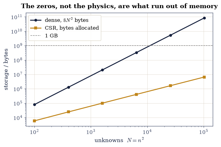
Fig. 31 Storage cost of the discrete \(-\nabla^2\) of Eq. 33 on an \(n\times n\) grid, against the number of unknowns \(N=n^2\): the dense array of doubles (dark, \(8N^2\) bytes) grows quadratically and crosses one gigabyte (dashed) near \(N=10^4\), while the compressed-sparse-row arrays actually allocated (amber) grow linearly with the \(5N\) non-zeros; at \(N=320^2\) the same operator costs 6.5 MB sparse and would cost 84 GB dense.

Validation 5

✓  the sparse assembly reproduces the analytic spectrum of −∇²   [max|Δ| = 5.45697e-12 (rtol=1e-10, atol=1e-09)]
✓  the five-point stencil gives exactly 5n²−4n non-zeros, never more than five per row   [nnz = 1920, 5n²−4n = 1920]
✓  at n = 320 the discarded zeros would have cost over 1000× the matrix itself   [83.9 GB dense vs 6.5 MB sparse (12830×)]

True

Exercise 6 — Krylov subspaces: Lanczos, and shift-invert for the smallest

The dense spectrum taken in Exercise 5 was affordable only because \(N=400\); the same call at \(n=320\) would ask for 84 GB and \(O(N^3)\) work for numbers we do not want. A Krylov method, Eq. 30, asks the operator for nothing but products \(A\mathbf x\). For symmetric \(A\) the Lanczos iteration builds an orthonormal basis \(\mathbf q_1,\mathbf q_2,\dots\) of \(\mathcal K_k(A,\mathbf q_1)\) with a three-term recurrence,

(35)\[A\mathbf q_j = \beta_{j-1}\mathbf q_{j-1} + \alpha_j\mathbf q_j + \beta_j\mathbf q_{j+1}, \qquad \alpha_j = \mathbf q_j^\top A\mathbf q_j, \qquad \beta_j = \lVert\mathbf w_j\rVert,\]

where \(\mathbf w_j\) is what remains of \(A\mathbf q_j\) once the two previous basis vectors are projected out, and \(\mathbf q_{j+1}=\mathbf w_j/\beta_j\). Only three terms appear because symmetry forces the projected matrix \(T_k=Q_k^\top A Q_k\) to be tridiagonal, with the \(\alpha_j\) on the diagonal and the \(\beta_j\) beside it. Its eigenvalues, the Ritz values, then cost almost nothing: a \(k\times k\) symmetric tridiagonal eigensolve, with \(k\ll N\).

In exact arithmetic the recurrence keeps the \(\mathbf q_j\) orthogonal by itself. In floating point it does not: as a Ritz value converges, rounding leaks its eigendirection back into the basis and the iteration reports the same eigenvalue several times over, the “ghost” eigenvalues, a loss of orthogonality of exactly the kind §0.1 warns about. Subtracting the stored basis off once per step (full reorthogonalization) is the honest fix at this scale.

Lanczos converging from the outside in is a problem whenever the physics wants the bottom of the spectrum, because “outside” is measured against the whole spectral width: for the Laplacian above \(\lambda_{\min}\) and its neighbour are separated by under a hundredth of the range, while \(\lambda_{\max}\) sits alone at the far edge. Shift-invert repairs this by running the iteration on a different operator, since the eigenvalues of \((A-\sigma I)^{-1}\) are

(36)\[\mu_i = \frac{1}{\lambda_i - \sigma},\]

so whichever \(\lambda_i\) lie nearest the shift \(\sigma\) become the largest \(\mu_i\) by a wide margin, and the outside-in bias now points where we want it. Taking \(\sigma=0\) targets the smallest eigenvalues, which is what eigsh(A_rect, k=8, sigma=0.0) means in §3.9. The price is one sparse factorization of \(A-\sigma I\), formed once and reused at every iteration: a real cost, and still nothing beside a dense \(O(N^3)\) eigendecomposition. The alternative idiom which="SA" skips the factorization and asks for the smallest algebraic eigenvalues directly, which is what §7.19 and §8.2 use; it reaches the same answer through more iterations, and the timings below measure the difference.

1. Write lanczos(A, v0, k) implementing Eq. 35 and returning the diagonal alpha (length \(k\)) and off-diagonal beta (length \(k-1\)) of \(T_k\). The operator must be touched only through A @ q; reorthogonalize each new \(\mathbf w_j\) against the whole stored basis before normalizing. Write this one yourself — the implementation is the lesson.

2. Run it on the laplacian_2d(20) operator of Exercise 5 from the starting vector numpy.random.default_rng(0).standard_normal(400), for \(k=5,10,20,30,40\). Assemble \(T_k\) with numpy.diag on the three bands, take scipy.linalg.eigvalsh(T_k), and track three relative errors against Exercise 5’s dense spectrum: the extreme Ritz values against \(\lambda_{\min}\) and \(\lambda_{\max}\), and the closest Ritz value to the median eigenvalue \(\lambda_{N/2}\) (Fig. 32).

3. Take the six smallest eigenvalues twice, by eigsh(A, k=6, which="SA") and by shift-invert eigsh(A, k=6, sigma=0.0), and check both against the first six of the dense spectrum. Then quantify Eq. 36: compare the relative separation of the target eigenvalue, \((\lambda_2-\lambda_1)/(\lambda_N-\lambda_1)\), with the same quantity for the \(\mu_i=1/\lambda_i\).

4. Time all three routes (dense eigvalsh on .toarray(), which="SA", and shift-invert) for \(n=20,30,40,50,60\) with time.perf_counter, and plot the wall-clock cost against \(N\) with an \(N^3\) reference slope (Fig. 33).

   k   rel.err λ_min   rel.err λ_max   rel.err λ_median
   5        1.01e+01        5.34e-02           1.59e-02
  10        2.74e+00        1.49e-02           1.02e-01
  20        4.38e-01        2.29e-03           5.10e-02
  30        8.66e-03        6.01e-05           3.41e-02
  40        7.72e-05        5.84e-07           1.99e-02
six smallest, which='SA'  = [19.7024 49.036  49.036  78.3696 97.1967 97.1967]
six smallest, σ = 0       = [19.7024 49.036  49.036  78.3696 97.1967 97.1967]
dense reference           = [19.7024 49.036  49.036  78.3696 97.1967 97.1967]
relative separation of the target: 0.0084 in A, 0.6016 in A⁻¹  (72× wider)

     N    dense/s     SA/s   σ=0/s     dense/(σ=0)
   400     0.009    0.014   0.007              1×
   900     0.067    0.027   0.011              6×
  1600     0.248    0.048   0.018             14×
  2500     0.829    0.068   0.028             29×
  3600     2.563    0.089   0.039             65×

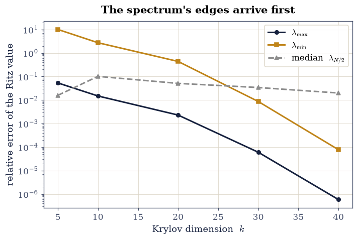
Fig. 32 Lanczos converges from the outside in. Relative error of the Ritz values of Eq. 35 against the dense spectrum of the \(N=400\) discrete \(-\nabla^2\), as a function of the Krylov dimension \(k\): the extremes \(\lambda_{\max}\) (dark) and \(\lambda_{\min}\) (amber) fall geometrically and are pinned to better than \(10^{-4}\) by \(k=40\), a tenth of the matrix dimension, while the best Ritz approximation to the median eigenvalue \(\lambda_{N/2}\) (grey) is still stuck near a percent.

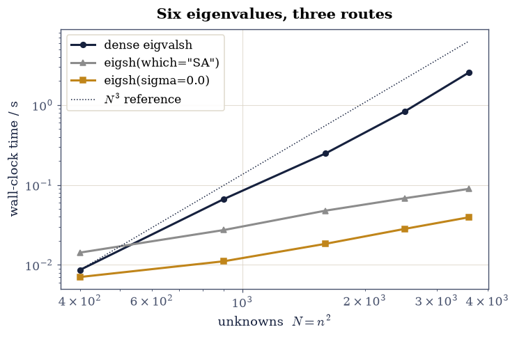
Fig. 33 Wall-clock cost of three routes to the six smallest eigenvalues of the discrete \(-\nabla^2\), against the number of unknowns \(N\): the dense eigvalsh on the filled-in array (dark) tracks the \(N^3\) reference slope (dotted) because it computes the entire spectrum by similarity transformations, whereas the Krylov solvers eigsh(which="SA") (grey) and shift-invert eigsh(sigma=0.0) (amber) build only a small Krylov subspace and stay near-linear; the shift replaces the extra iterations which="SA" spends with a single sparse factorization.

Validation 6

✓  Lanczos converges from the outside in: at k = 40 both spectral extremes are pinned while the middle of the spectrum is not   [rel. error λ_min 7.7e-05, λ_max 5.8e-07, median 2.0e-02]
✓  shift-invert eigsh(σ=0) returns the six smallest eigenvalues of the dense solve   [max|Δ| = 3.06244e-12 (rtol=1e-08, atol=1e-09)]
✓  eigsh(which='SA') reaches the same six without a factorization   [max|Δ| = 3.2685e-12 (rtol=1e-08, atol=1e-09)]
✓  shift-invert widens the target eigenvalue's relative separation by an order of magnitude or more, which is why it converges   [0.0084 → 0.6016  (72×)]
✓  at N = 3600 the dense eigendecomposition costs several times the sparse shift-invert solve (a wall-clock check: the margin, not the number, is the claim)   [dense 2.563 s vs σ=0 0.039 s (65×)]

True

Exercise 7 — The SVD: definition and geometry (worked animation)

The SVD, Eq. 31, applies to any matrix, and its content is geometric. We take two explicit matrices. First, to check the algebra, the \(3\times2\)

\[\begin{split} A = \begin{bmatrix} 3 & 1 \\ 1 & 3 \\ 2 & 2 \end{bmatrix}: \end{split}\]

1. Compute \(U,\Sigma,V^\top\) with scipy.linalg.svd, verify the reconstruction \(A=U\Sigma V^\top\), and confirm \(\sigma_i=\sqrt{\lambda_i(A^\top A)}\) (scipy.linalg.eigvalsh on \(A^\top A\)).

Then, to see the geometry, take the \(2\times2\)

\[\begin{split} B = \begin{bmatrix} 3 & 1 \\ 0 & 2 \end{bmatrix}, \end{split}\]

which sends the unit circle to an ellipse.

2. Animate the map decomposed into its three SVD acts (\(V^\top\) rotates, \(\Sigma\) stretches along the axes, \(U\) rotates) with FuncAnimation.

3. Confirm the resulting ellipse has semi-axes exactly \(\sigma_1,\sigma_2\) (Fig. 34) — the claim the validation checks against the animated points.

singular values     = [4.899 2.   ]
√eig(AᵀA) (desc)    = [4.899 2.   ]

Validation 7a — the SVD algebra

✓  A = UΣVᵀ reconstructs A   [max|Δ| = 8.88178e-16 (rtol=1e-06, atol=1e-10)]
✓  σ = √eig(AᵀA)   [max|Δ| = 4.44089e-16 (rtol=1e-06, atol=1e-10)]

True

Now the geometry of \(B=\begin{bmatrix}3&1\\0&2\end{bmatrix}\). Fix the SVD sign freedom so both \(U\) and \(V^\top\) are proper rotations, then animate the unit circle through the three acts.

Once Loop Reflect

Fig. 34 Animation of the geometric action of \(B=\bigl[\begin{smallmatrix}3&1\\0&2\end{smallmatrix}\bigr]\) on the unit circle, decomposed by its SVD \(B=U\Sigma V^\top\) into three acts: \(V^\top\) rotates the circle, \(\Sigma\) stretches it along the axes into an ellipse, and \(U\) rotates that ellipse into place. The final ellipse’s semi-axes are the singular values \(\sigma_1,\sigma_2\) (amber); every linear map is rotate–scale–rotate.

Validation 7b — the geometry of the data

✓  the unit circle maps to an ellipse with semi-axes σᵢ   [max|Δ| = 1.11417e-06 (rtol=0.001, atol=1e-09)]

True

Exercise 8 — Low-rank approximation and Eckart–Young

Here is the centrepiece. Eckart–Young, Eq. 32, says the truncated SVD is the best rank-\(k\) approximation and that its spectral-norm error is exactly the first singular value we discarded, \(\sigma_{k+1}\). We test this on a fixed, reproducible matrix: the \(8\times6\) matrix \(B\) whose entries are numpy.random.default_rng(0).standard_normal((8, 6)) (seed 0, shape \(8\times6\), stated so the result is unambiguous).

1. For \(k=1,2,3,4\) form the rank-\(k\) truncation \(\sum_{i\le k}\sigma_i\mathbf u_i\mathbf v_i^\top\) from the scipy.linalg.svd factors.

2. Confirm its spectral-norm error (numpy.linalg.norm(..., 2)) equals \(\sigma_{k+1}\) (Fig. 35).

rank-k spectral error : [3.3879 2.2443 1.9781 1.3504]
σ_(k+1)               : [3.3879 2.2443 1.9781 1.3504]

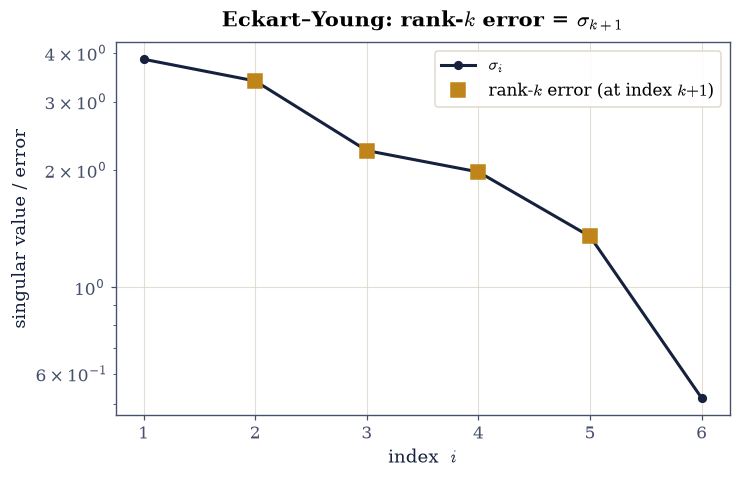
Fig. 35 Eckart–Young for the \(8\times6\) matrix \(B\) with entries default_rng(0).standard_normal((8,6)): the singular-value spectrum \(\sigma_i\) (dark) and, overlaid, the measured spectral-norm error of the rank-\(k\) truncated SVD (amber circles) sitting exactly on \(\sigma_{k+1}\) — the best rank-\(k\) approximation errs by precisely the first discarded singular value.

Validation 8

✓  the rank-k truncated-SVD error equals σ_(k+1) (Eckart–Young)   [max|Δ| = 2.22045e-15 (rtol=1e-06, atol=1e-09)]

True

Exercise 9 — Compression: a low-rank matrix in noise (student exercise)

Real data is rarely exactly low-rank, but it is often nearly so, and the SVD exposes that at a glance. The matrix to analyse is the explicit

\[ M_{ij} = \sin(2\pi x_i) + x_i\,g_j + 0.01\,\eta_{ij}, \]

with \(x=\texttt{linspace}(0,1,40)\), \(g=\texttt{linspace}(1,2,30)\), and noise \(\eta=\texttt{default\_rng(0).standard\_normal((40,30))}\) (seed 0, shape \(40\times30\)). The first two terms are each a rank-1 outer product, so \(M\) is rank 2 plus a small noise floor.

1. Build \(M\) from those three pieces: the two rank-1 outer products and the scaled noise.

2. Compute the singular values with scipy.linalg.svd and see two dominate before a cliff.

3. Reconstruct the rank-2 matrix from the truncated factors (broadcast the top two singular values into the product) and check the noise is gone.

4. Quantify \(\sigma_3/\sigma_1\) as the effective-rank signal.

There is no animation here: this is a spectrum-and-reconstruction analysis, not motion; a ✗ points at the construction of \(M\) or the truncation.

first five singular values = [30.9169  4.3457  0.1071  0.0972  0.0969]
σ₃/σ₁ = 0.0035   (effective rank ≈ 2)
rank-2 captures 99.99% of the Frobenius norm

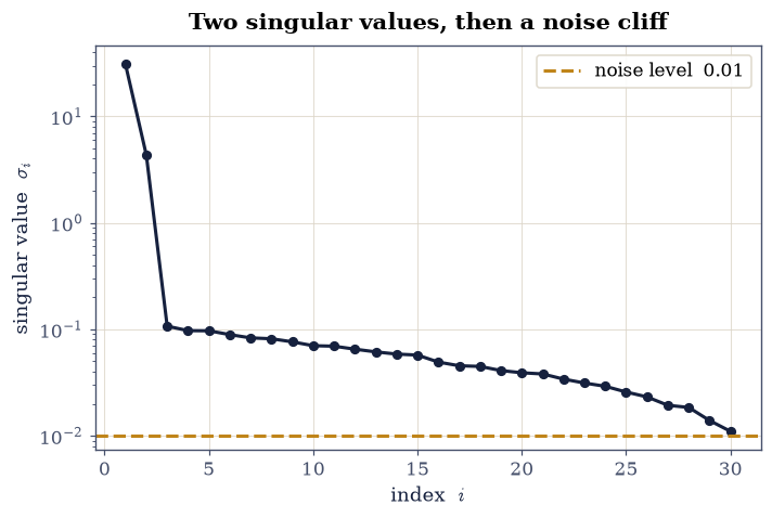
Fig. 36 Singular-value spectrum of the \(40\times30\) matrix \(M_{ij}=\sin(2\pi x_i)+x_i g_j+0.01\eta_{ij}\) (seed 0): two singular values dominate and then the spectrum falls off a cliff into a flat noise floor, so \(M\) is effectively rank 2. Keeping the top two singular triples reconstructs the signal and discards the noise — the SVD reads off the effective rank.

Validation 9

✓  the matrix is effectively rank 2: the noise lives in the tiny tail of the spectrum   [σ₃/σ₁ = 0.0035]

True

Exercise 10 — The SVD → tensor networks (synthesis, and an honest horizon)

The move just made in Exercise 9 (keep the few large singular values, discard the small tail) is, almost word for word, how the tensor networks of many-body quantum physics are built. A quantum state of \(N\) particles lives in a Hilbert space of dimension \(2^N\), hopelessly large; but a physical state (a ground state of a local Hamiltonian) has, across any bipartition, an entanglement spectrum (the singular values of the state reshaped into a matrix) that decays rapidly, just like the noisy matrix above. A matrix-product state (MPS) exploits exactly this: truncate each bond’s SVD to the largest few singular values (the “bond dimension”), and the \(2^N\) cost collapses to something linear in \(N\). DMRG is the algorithm that does this truncation variationally to find ground states.

No notebook in this course builds an MPS, and it is worth being exact about where the course does stop. §7.19 measures the entanglement entropy of a spin chain and finds it saturating, which is the evidence that a small bond dimension can suffice; §8.13 diagonalizes many-body Hamiltonians exactly and names DMRG among the methods that reach the sizes exact diagonalization cannot. Both point outward, neither implements. For the algorithms themselves the standard entry point is Schollwöck’s review of DMRG in the language of matrix product states. What belongs here is the principle they rest on. Keeping just the top two singular triples of the Exercise-9 matrix already captures essentially all of its Frobenius norm: the same statement, for our toy matrix, as “a low-entanglement state is well approximated by a small bond dimension.”

top-2 singular triples capture 99.99% of ‖M‖_F

Validation 10

✓  keeping a few singular values captures almost all of the matrix — the principle behind tensor-network (MPS/DMRG) compression   [captured fraction = 0.9999]

True

Notebook summary

• The symmetric eigenproblem and the spectral theorem (\(A=V\Lambda V^\top\), \(V^\top V=I\)), why the characteristic polynomial is the wrong tool, and the QR algorithm built from scratch; the generalized eigenproblem (callback to §2.7).

• Sparsity and Krylov methods. The five-point Laplacian on a \(20\times20\) grid has \(5n^2-4n=1920\) non-zeros in \(N^2=160{,}000\) entries, a density of \(0.012\); at \(n=320\) the dense array would cost 84 GB against 6.5 MB stored sparsely. A hand-written Lanczos iteration, which touches the matrix only through \(A\mathbf x\), pins both spectral extremes to a relative \(10^{-4}\) by Krylov dimension \(k=40\) out of \(N=400\) while the middle of the spectrum is still wrong in the second digit, and shift-invert turns that outside-in bias toward the smallest eigenvalues by widening their relative separation from \(0.008\) to \(0.60\), a factor of 72.

• The SVD (\(A=U\Sigma V^\top\), \(\sigma=\sqrt{\mathrm{eig}(A^\top A)}\)), low-rank approximation and the Eckart–Young theorem, compression in noise, and the SVD as the seed of tensor-network methods.

Outlook

• Non-symmetric eigenproblems. Complex spectra, non-orthogonal eigenvectors, and defective matrices with a Jordan form: numerically delicate, and a reason the symmetric case is so prized.

• Power and inverse iteration. The one-vector ancestors of Lanczos, which keep only the newest \(A^k\mathbf b\) instead of the whole Krylov subspace and converge correspondingly slower; the seed of PageRank.

• Arnoldi, and life without symmetry. Drop \(A=A^\top\) and the three-term recurrence becomes a full Hessenberg one: that is scipy.sparse.linalg.eigs, with complex Ritz values and no guarantee of an orthonormal eigenbasis.

• Preconditioning. Shift-invert is one way to reshape a spectrum in favour of the eigenvalues one wants; LOBPCG and preconditioned conjugate gradient (the iterative solvers named in the Outlook of §0.4) are the others, and they are what make the largest ground-state problems move at all.

• PCA is the SVD of a data matrix: a forward link to the least-squares fitting of §0.8, where the SVD also gives the pseudoinverse for rank-deficient problems.

• Tensor networks (MPS/DMRG) take the Eckart–Young truncation to many-body quantum states. This course goes as far as the evidence for them and stops there: no notebook builds an MPS or runs DMRG (outward, named — Schollwöck’s review is the way in).

References

[GVL13]

Gene H. Golub and Charles F. Van Loan. Matrix Computations. Johns Hopkins University Press, 4 edition, 2013.

[TB97]

Lloyd N. Trefethen and David Bau. Numerical Linear Algebra. Society for Industrial and Applied Mathematics (SIAM), 1997.

Take this notebook with you

Use the download button (↓) in the toolbar above to save this notebook and run it yourself. The published notebooks ship without worked solutions; if you would like the reference solutions — to teach from or to check your own work — get in touch: hello@ramador.me.