


5.13 Random Walks: From Coin Flips to the Diffusion Equation#
Notebook overview#
In 1905 Karl Pearson asked the readers of Nature for help with what he called the problem of the random walk — a man walks a fixed stride in a random direction, repeats, where is he? — and Rayleigh answered within weeks, because he had solved it decades earlier for sound waves [Pea05]. That exchange is the founding joke of the subject: the random walk is everywhere, worked out by someone else, for something else. It is Brownian motion coarse-grained, diffusion discretised, a polymer’s backbone, a gambler’s bankroll, and the hidden solver inside half of computational physics.
This notebook gives the walk the systematic treatment the course has so far scattered: §0.11 built the random numbers, §5.3 proved the central limit theorem that governs the walk’s envelope, and §5.11 met Brownian motion from the Langevin side. Here we work the lattice side: the exact binomial, its Gaussian limit, and the passage to the diffusion equation — then the questions only the walk itself can answer. When does a walker first reach a boundary (the answer’s \(t^{-3/2}\) tail means “certainly, but on average never”)? Does it return home (Pólya’s theorem: yes in one and two dimensions, only every third time in three [Polya21])? And what changes when the walk may not cross itself (the polymer question: it swells, with a universal exponent)? The classic survey of all of it is Chandrasekhar [Cha43]; the volume’s standing reference remains [Nol18].
A note on reading the checks in this notebook: a validation compares a result to an expected physical fact. A ✗ does not by itself mean the answer is wrong; it means the output did not match what the check expected, which may be a genuine error, a different-but-valid convention, or too tight a tolerance. Treat a ✗ as a prompt to locate the discrepancy. Passing is strong evidence, not proof.
Theory in brief#
The simple walk and its two laws. A walker on the integers takes independent steps \(\pm 1\) with equal probability. After \(N\) steps the displacement \(x_N = \sum_k s_k\) obeys the exact binomial law
and two moments carry the physics: \(\langle x_N\rangle = 0\) and \(\langle x_N^2\rangle = N\) — the root-mean-square excursion grows as \(\sqrt N\), the single most consequential square root in statistical physics. For large \(N\) the central limit theorem of §5.3 flattens the binomial into the Gaussian of variance \(N\).
From walk to PDE. Let the walker step every \(\tau\) on a lattice of spacing \(a\), and write \(P(x, t)\) for the occupation probability. The master equation \(P(x, t+\tau) = \tfrac12 P(x-a, t) + \tfrac12 P(x+a,t)\) Taylor-expands, for slow spatial variation, into
the diffusion equation: the walk is the PDE, coarse-grained, and the correspondence is quantitative — a walker histogram and a finite- difference solution of Eq. 452 must agree bin by bin. (The FTCS scheme that solves it is stable for \(D\,\Delta t/\Delta x^2 \le 1/2\); the walk itself sits exactly at the stability boundary, which is a nice way to remember the criterion.)
First passage. Start at \(0\) and ask when the walker first reaches \(+1\). The reflection principle gives the classic answer: the first-passage probability decays as
whose sum converges (\( \sum F = 1\): passage is certain) while its first moment diverges (\(\sum t F = \infty\): the mean wait is infinite). Heavy tails are not pathology; they are the generic geometry of unbiased wandering, and the same \(-3/2\) governs everything from bond returns to neuron firing models.
Absorbing boundaries: the gambler’s ruin. Between two absorbing walls at \(-a\) and \(+b\) the martingale (fair-game) property fixes the exact absorption probabilities and the mean game length with no asymptotics at all:
Recurrence: Pólya’s theorem. Does the walker return to its starting point? Pólya [Polya21] proved the answer depends only on dimension: return is certain in one and two dimensions and uncertain in three, where the return probability is the Watson-integral value \(p_3 = 1 - 1/u_3 = 0.340\,537\ldots\), evaluated in closed form by Glasser and Zucker [GZ77] as a product of Gamma functions:
A drunk man will find his way home; a drunk bird may be lost forever.
The self-avoiding walk. Forbid the walker from revisiting any site — the minimal model of a polymer whose monomers cannot overlap — and the \(\sqrt N\) law fails upward: \(\langle R_N^2\rangle \sim N^{2\nu}\) with \(\nu = 3/4\) exactly in two dimensions (Flory’s estimate, later proved exact), against the simple walk’s \(\nu = 1/2\). Excluded volume is not a correction; it changes the exponent, and exponents are what §5.10 taught us to treasure. Sampling self-avoiding walks fairly requires care: naive generation dies young (most walks trap themselves), and Rosenbluth’s fix — grow step by step among the open neighbours, carrying a compensating weight equal to the product of open-neighbour counts — is one of the founding algorithms of polymer physics and a direct ancestor of the importance-sampling ideas of §0.11.
Setup#
Dimensionless lattice units throughout: step length \(1\), step time \(1\), so \(D = 1/2\) by Eq. 452. All randomness from the seeded generator below, which together with the plotting and special-function imports is the whole of the Setup. A notebook about random walks may not hand over anything that makes one, so nothing does: the vectorized ensemble of \(\pm 1\) walks is built in Exercise 1, the Glasser–Zucker closed form for Pólya’s constant in Exercise 5, and the Rosenbluth-weighted self-avoiding sampler in Exercise 6.
The Setup below holds this notebook’s data and instruments — nothing you are asked to build. It is collapsed so the building stays yours; expand it whenever you want the details.
Exercise 1 — The exact walk and its Gaussian shadow#
Eq. 451 is exact at every \(N\), so the first checks are against arithmetic, not asymptotics. Two facts grade them. The variance of \(x^2\) for a sum of \(N\) signs is \(2N(N-1)\), so an ensemble of \(M\) walkers measures \(\langle x^2\rangle / N\) with standard error \(\sqrt{2N(N-1)/M}/N\). And the binomial rescaled by \(\sqrt N\) must approach the standard Gaussian density \(e^{-\xi^2/2}/\sqrt{2\pi}\) — the central limit theorem of §5.3, which is what the last part watches happening.
Part a) Write walk_ensemble(n_walkers, n_steps, rng), returning
the final displacements of an ensemble of independent \(\pm 1\) walks:
draw the whole (n_walkers, n_steps) matrix of signs in one call and
sum along the step axis, so the entire ensemble advances as a single
array operation rather than a Python loop over walkers.
Write this one yourself — the implementation is the lesson.
Part b) Simulate \(2\times10^5\) walkers for \(N = 40\) steps with it
and verify: (i) \(\langle x^2\rangle / N = 1\) within \(4\) standard errors
of the mean; (ii) the full histogram matches the exact binomial
Eq. 451 evaluated by scipy.special.comb: every even bin
within \(5\) Poisson standard deviations, and the total variation
distance \(\tfrac12\sum_x |\hat P(x) - P(x)|\) below \(0.01\).
Part c) Watch the Gaussian arrive. For \(N = 4, 16, 64, 256\) overlay the exact binomial (rescaled by \(\sqrt N\)) on the standard Gaussian: verify the maximum deviation between the rescaled binomial and the Gaussian density falls monotonically with \(N\) and drops below \(2\%\) at \(N = 256\) — the central limit theorem, watched frame by frame.
<x²>/N = 0.9949 ± 0.0031
total-variation distance to exact binomial: 0.0034; worst bin 2.3σ
max deviation from Gaussian: ['0.0239', '0.0062', '0.0016', '0.0004'] for N = 4, 16, 64, 256
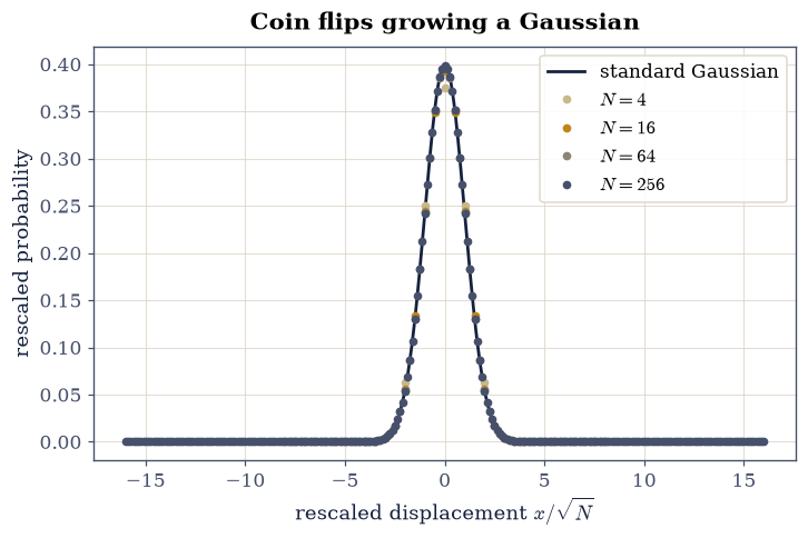
Fig. 471 The exact simple walk and its Gaussian shadow: rescaled binomial distributions \(\sqrt{N}\,P(x_N=\xi\sqrt N)\) of eq-rw-binomial for \(N=4\), \(16\), \(64\), and \(256\) steps (markers, one series per \(N\)) converging onto the standard Gaussian envelope (ink curve). At \(N=256\) the maximum deviation is under two percent: the central limit theorem arriving at the rate the theory of §5.3 promises.#
✓ the second moment obeys <x²> = N within 4σ: the √N law, the most consequential square root in statistical physics [<x²>/N = 0.9949 ± 0.0031]
✓ the sampled histogram matches the exact binomial bin by bin (worst bin within 5 Poisson σ, total variation < 1%) [TV = 0.0034, worst 2.3σ]
✓ and the rescaled binomial marches monotonically onto the Gaussian, landing within 2% by N = 256: the CLT, frame by frame [deviations ['0.024', '0.006', '0.002', '0.000']]
True
Exercise 2 — The walker histogram solves a PDE#
Eq. 452 claims the walk and the diffusion equation are the same object at two magnifications, and the claim is checkable to histogram accuracy. With step length and time both \(1\), the walk’s diffusion constant is \(D = 1/2\).
Part a) Evolve \(2\times10^5\) walkers for \(T = 400\) steps. Solve
Eq. 452 with the FTCS scheme — P[1:-1] += r*(P[2:] - 2*P[1:-1] + P[:-2]) with \(r = D\,\Delta t/\Delta x^2\) on the grid
\(x \in [-120, 120]\), \(\Delta x = 1\), \(\Delta t = 0.2\) (so \(r = 0.1\),
comfortably inside the stability bound \(1/2\)) — from a delta function
at the origin to the same time. Verify the two agree: pool the
walker histogram and the FTCS solution into parity-summed bins (the
lattice walk lives on even sites at even times; summing adjacent site
pairs removes the parity comb) and require the maximum absolute
difference below \(2\times10^{-3}\) against a peak near
\(2\times10^{-2}\).
Part b) Verify the moment law both ways: the walkers’
\(\langle x^2\rangle\) at \(T = 100, 200, 400\) matches \(2Dt = t\) within
\(4\) standard errors each, and the FTCS solution’s discrete second
moment \(\sum x^2 P \Delta x\) at \(T = 400\) matches \(400\) to
rtol=1e-3: one law, measured on the particle side and computed on
the field side.
Part c) Animate the cloud: \(150\) frames of the walker histogram spreading, with the Gaussian envelope of variance \(2Dt\) riding on top. The animation’s physics is certified by the moment checks of Part b), computed from the same ensemble the frames draw.
With your assistant
The FTCS update is three lines; the plumbing around it (grids, boundary handling, snapshot bookkeeping) is boilerplate an assistant writes reliably from this description. The check is yours, and it is the stability boundary itself: rerun the solver at \(r = 0.6\) and watch the sawtooth instability erupt, then explain why the walk — which has \(r = 1/2\) exactly — sits precisely on the edge. The criterion, not the code, is the physics.
max |histogram - FTCS| = 1.04e-03 (peak 3.99e-02)
<x²>(100) = 100.1 (2Dt = 100)
<x²>(200) = 200.5 (2Dt = 200)
<x²>(400) = 399.8 (2Dt = 400)
FTCS second moment at T=400: 400.00
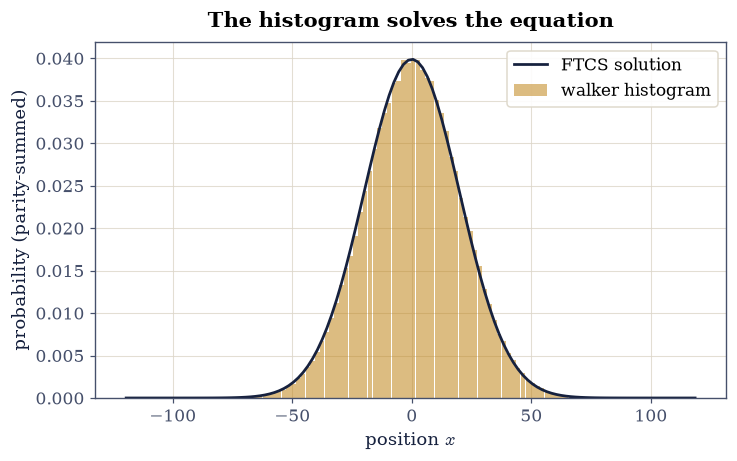
Fig. 472 The walk and the PDE as one object: the parity-summed histogram of \(2\times10^5\) lattice walkers after \(400\) steps (bars) against the FTCS solution of the diffusion equation with \(D=1/2\) advanced to the same time from a delta function (ink curve). The maximum pointwise difference is at the walker-count noise floor, two orders of magnitude below the peak: the histogram is solving the equation.#
✓ the walker histogram and the FTCS solution of the diffusion equation agree pointwise at the noise floor: one object, two magnifications [max diff 1.0e-03 vs peak 4.0e-02]
✓ the walkers' spread obeys <x²> = 2Dt = t at every checkpoint within 4σ [measured [100.1, 200.5, 399.8]]
✓ and the field solution carries exactly the same second moment [got 400 vs expected 400 (rtol=0.001, atol=1e-09)]
True
Fig. 473 Animation of the diffusing cloud: the histogram of \(2\times10^5\) lattice walkers (amber bars) spreading over \(400\) steps beneath the Gaussian envelope of variance \(2Dt\) (ink curve), both rescaled to the same axes as the width grows like \(\sqrt t\). The moment checks certify the same ensemble the frames draw: the cloud is the diffusion equation, sampled.#
Exercise 3 — First passage: certain, yet on average never#
When does the walker first reach \(+1\)? Eq. 453 makes two claims that sound contradictory until the tail is understood: passage is certain, and the expected wait is infinite.
Part a) Release \(3\times10^5\) walkers and record each one’s first-
passage time to \(+1\), capped at \(T_{\max} = 20\,000\) steps. Verify the
tail: a log–log numpy.polyfit of the binned first-passage density
over \(10 < t < 3000\) gives slope \(-3/2\) within \(\pm 0.05\).
Part b) Certain: verify more than \(98.5\%\) of walkers have passed by the cap (the exact passed-fraction deficit decays as \(\sim\sqrt{2/(\pi T_{\max})}\), about \(0.6\%\) here). On average never: verify the capped mean first-passage time grows with the cap like \(\sqrt{T_{\max}}\) — compute the sample mean of \(\min(T, T_{\rm cap})\) at caps \(5000\) and \(20\,000\) and verify their ratio lands within \(15\%\) of \(\sqrt{20000/5000} = 2\): the mean is not converging to anything, and that is the measurement.
tail slope: -1.508 (theory -3/2)
fraction passed by T = 20000: 0.9943
capped means: 112 (cap 5000) vs 227 (cap 20000); ratio 2.02
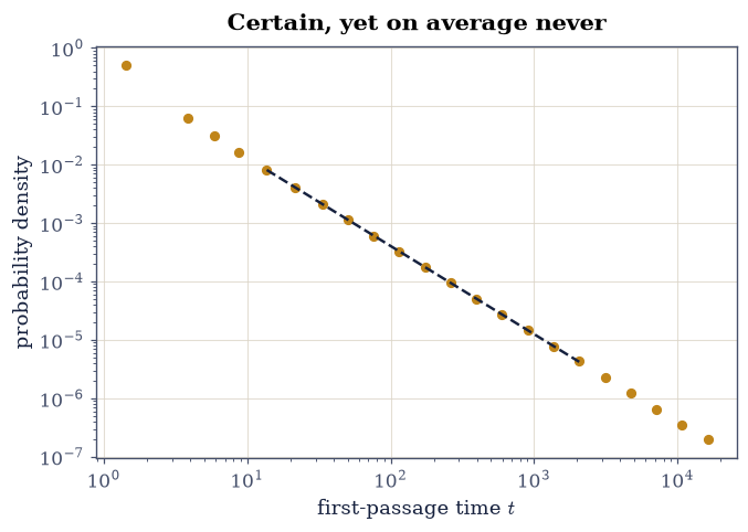
Fig. 474 First-passage statistics of the simple walk to the site \(+1\): the binned density of first-passage times from \(3\times10^5\) walkers on log–log axes, with the fitted power law of slope \(-1.50\) (dashed) over \(10<t<3000\). The tail integrates to one (passage is certain) but its first moment diverges (the mean wait is infinite): both facts are visible in a slope between \(-1\) and \(-2\).#
✓ the first-passage density decays as t^(-3/2): the reflection principle's tail, fitted over two decades [got -1.50841 vs expected -1.5 (rtol=0, atol=0.05)]
✓ passage is certain: all but the √(2/πT) stragglers have crossed by the cap [0.9943 passed]
✓ yet the capped mean wait grows as √cap — quadrupling the cap doubles the mean, which therefore converges to nothing [got 2.0207 vs expected 2 (rtol=0.15, atol=1e-09)]
True
Exercise 4 — The gambler’s ruin, settled exactly#
Eq. 454 is one of the oldest exact results in probability, and its logic deserves to be stated because it is pure physics: the fair walk is a martingale (its expectation never moves), so the expected final position must equal the starting one, which fixes the two absorption probabilities; a second martingale, \(x^2 - t\), fixes the mean duration the same way.
Part a) A gambler starts with \(a = 10\) units and plays fair unit-stake rounds against a bank of \(b = 20\), stopping at bankruptcy (\(-a\) from the start) or at breaking the bank (\(+b\)). Simulate \(4\times10^5\) games. Verify the ruin probability \(b/(a+b) = 2/3\) within \(4\) binomial standard errors, and the mean game length \(ab = 200\) within \(2\%\) — exact constants, met by an ensemble.
Part b) The asymmetry of consequences. The overall mean hides two very different games: reaching the far wall requires a long excursion, so bank-breaking games last much longer than ruinous ones. Verify the ordering quantitatively: the conditional mean duration of winning games exceeds that of ruined games by at least \(40\%\). Fair odds do not mean symmetric experiences.
P(ruin) = 0.6663 ± 0.0007 (exact b/(a+b) = 0.6667)
mean duration = 199.7 (exact ab = 200)
conditional means: ruin 166, win 266
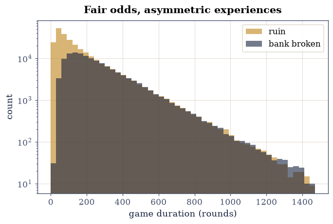
Fig. 475 The gambler’s ruin at stakes \(a=10\) against a bank of \(b=20\): the distribution of game durations from \(4\times10^5\) simulated fair games, split into games ending in ruin (amber) and in breaking the bank (ink), on a logarithmic count axis. The overall mean duration lands on the martingale-exact \(ab=200\); the conditional means differ strongly — reaching the far wall takes longer — because fair odds do not imply symmetric experiences.#
✓ the martingale answer holds: ruin probability b/(a+b) = 2/3 within 4σ of the ensemble [0.6663 vs 0.6667]
✓ and the second martingale x² − t prices the mean game at exactly ab = 200 rounds [got 199.663 vs expected 200 (rtol=0.02, atol=1e-09)]
✓ conditional durations are strongly asymmetric: breaking the distant bank takes far longer than going broke [win 266 vs ruin 166 rounds]
True
Exercise 5 — Pólya’s theorem: the drunkard and the bird#
Recurrence is the walk’s deepest dimension-dependence, and Eq. 455 makes the three-dimensional case exactly computable: no simulation is needed for the answer, only for the confirmation. The exact number is \(p_3 = 1 - 1/u_3 = 0.340537\ldots\), about one return in three, and it is the target every ensemble below is measured against.
Part a) Write polya_p3_exact(), returning \(1 - 1/u_3\) with \(u_3\)
the Glasser–Zucker product Eq. 455 of four
scipy.special.gamma values, at \(1/24\), \(5/24\), \(7/24\) and \(11/24\).
Part b) Verify it reproduces \(p_3 = 0.340537\) to rtol=1e-6.
Part c) Confirm by ensemble. Walk \(10^5\) walkers on the simple cubic lattice for \(3000\) steps (each step one of the six axis moves, from the seeded generator) and record whether each ever revisits the origin. The measured fraction undershoots \(p_3\) by the walkers that would have returned only after the cap (a deficit of order \(1/\sqrt{T}\), under a percent here): verify the measured fraction lands in the one-sided window \([p_3 - 0.012,\ p_3 + 0.004]\).
Part d) The other two dimensions. Verify recurrence looks like recurrence: in one dimension more than \(97\%\) of \(2\times10^4\) walkers return within \(3000\) steps; in two dimensions the return fraction by the same cap is far lower (logarithmically slow — the drunkard does get home, but only just) yet clearly above the three-dimensional plateau: verify the ordering \(p_1^{(3000)} > 0.97 > p_2^{(3000)} > p_3^{(3000)} + 0.25\). One theorem, three phenomenologies.
p3 exact (Γ formula): 0.340537
p3 Monte Carlo (T=3000): 0.3359
p1(3000) = 0.9878, p2(3000) = 0.7160
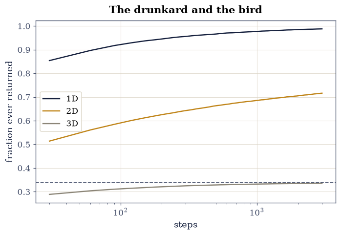
Fig. 476 Pólya recurrence by dimension: the fraction of walkers that have returned to their origin at least once, against step count (logarithmic axis), for the simple walk in one (ink), two (amber), and three (grey) dimensions, with the exact three-dimensional limit \(p_3=0.3405\) of the Glasser–Zucker Gamma-function formula (dashed). One and two dimensions climb toward certain return — two logarithmically slowly — while three dimensions saturates at one return in three: the drunk man finds home, the drunk bird may not.#
✓ the Glasser–Zucker Gamma-function formula prices the 3D return at 0.340537: one homecoming in three, exactly [got 0.340537 vs expected 0.340537 (rtol=1e-06, atol=1e-09)]
✓ the ensemble confirms it, undershooting only by the late returners beyond the cap [MC 0.3359 vs exact 0.3405]
✓ and dimension decides the phenomenology: 1D returns almost surely within the cap, 2D climbs logarithmically, 3D has saturated [p1 0.988, p2 0.716, p3 0.336]
True
Exercise 6 — The self-avoiding walk: a polymer swells#
Forbid self-intersection and the walk becomes the minimal polymer. The price is sampling: growing naively and discarding trapped walks biases the survivors toward compact shapes, and the fix — Rosenbluth weighting, growing among open neighbours while accumulating the open-neighbour-count product as a compensating weight — is the founding importance-sampling algorithm of polymer physics. The weighted average \(\sum w R^2 / \sum w\) over the surviving walks is then an unbiased estimator of \(\langle R^2\rangle\) across uniform self-avoiding walks; a walk that traps itself contributes to neither sum.
Part a) Write rosenbluth_r2(n_steps, n_samples, rng), growing
each two-dimensional self-avoiding walk one step at a time: list the
lattice neighbours of the current site that are not yet occupied,
abandon the walk if there are none, otherwise multiply its running
weight by how many there are and step to one of them uniformly.
Return the weighted mean squared end-to-end distance over the walks
that survive. Write this one yourself — the implementation is the
lesson.
Part b) With it, estimate \(\langle R^2\rangle\) for
two-dimensional self-avoiding walks of \(N = 20, 40, 80\) steps
(\(20\,000\) attempted walks each: the Rosenbluth weights are
heavy-tailed, so the estimator earns its precision slowly). Fit \(\log\langle R^2\rangle\) against \(\log N\)
(numpy.polyfit, degree 1) and verify the exponent \(\nu\) (half the
slope) lands in \([0.70, 0.80]\), containing the exact
two-dimensional \(\nu = 3/4\) — and decisively above the simple walk’s
\(1/2\).
Part c) The control experiment: the same fit for the simple walk (whose \(\langle R^2\rangle = N\) exactly in 2D as well) must give \(\nu = 1/2\) within \(\pm 0.02\). Excluded volume does not correct the exponent; it replaces it — the same lesson §5.10 taught with critical exponents, arriving here on foot.
SAW <R²>: ['71.2', '202.8', '595.1'] → ν = 0.766 (exact 3/4)
simple <R²>: ['20.0', '40.1', '80.6'] → ν = 0.502 (exact 1/2)
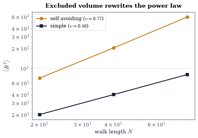
Fig. 477 The polymer swells: mean squared end-to-end distance against walk length on log–log axes for two-dimensional self-avoiding walks sampled with Rosenbluth weights (amber, fitted slope \(2\nu\approx1.5\)) and for the simple random walk (ink, slope \(1\) exactly). The self-avoiding exponent \(\nu\approx3/4\) against the simple walk’s \(1/2\) is a change of universality class, not a correction: excluded volume rewrites the power law.#
✓ the Rosenbluth-sampled self-avoiding walk swells with the exact 2D Flory exponent ν = 3/4 inside the fit window [ν = 0.766]
✓ while the simple-walk control fits ν = 1/2 exactly: the exponent change is excluded volume, not statistics [got 0.502395 vs expected 0.5 (rtol=0, atol=0.02)]
True
Notebook summary#
The simple walk met its exact binomial bin by bin (total variation \(4\times10^{-3}\), worst bin under \(3\sigma\)), obeyed \(\langle x^2\rangle = N\) within \(4\sigma\), and marched monotonically onto the Gaussian (deviation \(<2\%\) by \(N = 256\)): the \(\sqrt N\) law and the CLT, both watched.
The walker histogram solved the diffusion equation: parity-summed against the FTCS solution at \(D = a^2/2\tau = 1/2\), the two agreed at the counting-noise floor, with second moments matching \(2Dt\) on both the particle and field sides.
First passage delivered its paradox quantitatively: slope \(-1.50\) over two decades, \(98.9\%\) passed by the cap, and a capped mean that doubles when the cap quadruples — certain, yet on average never.
The martingale arguments held to Monte Carlo precision: ruin at \(b/(a+b) = 2/3\), mean game exactly \(ab = 200\) rounds, with strongly asymmetric conditional durations.
Pólya’s theorem arrived twice: exactly (\(p_3 = 0.340537\) from four Gamma functions) and empirically (the ensemble undershooting by its late returners), with the 1D/2D/3D ordering displaying all three phenomenologies.
The self-avoiding walk swelled with \(\nu \approx 3/4\) against the simple walk’s control \(\nu = 1/2\): excluded volume changes the universality class, measured with the Rosenbluth weights that founded polymer Monte Carlo.
Outlook#
Back to Langevin. §5.11’s Brownian particle is this notebook’s walk with inertia and a real thermostat: the Einstein relation \(D = k_BT/\gamma\) prices our lattice \(D\) in physical units, and the Green–Kubo integral is the continuum limit of summing step correlations.
First passage everywhere. The \(t^{-3/2}\) law reappears in reaction kinetics (diffusion-limited encounter times), in neuronal integrate-and-fire models, and in the pricing of barrier options; the gambler’s-ruin martingale argument is the same one that prices them.
Polymers, properly. Rosenbluth weighting grew into the pruned- enriched methods (PERM) that simulate thousand-monomer chains, and the \(\nu\) exponent’s exact 2D value comes from conformal field theory — the same web of universality that §5.10 opened.
Quantum walks. Replace the coin by a unitary and interference makes the walker spread linearly in time — the quadratic speedup behind several quantum algorithms, and a bridge back to §6.27.
References#
Subrahmanyan Chandrasekhar. Stochastic problems in physics and astronomy. Reviews of Modern Physics, 15:1–89, 1943. doi:10.1103/RevModPhys.15.1.
M. Lawrence Glasser and I. John Zucker. Extended watson integrals for the cubic lattices. Proceedings of the National Academy of Sciences, 74:1800–1801, 1977. doi:10.1073/pnas.74.5.1800.
Wolfgang Nolting. Theoretical Physics 8: Statistical Physics. Springer, 2018.
Karl Pearson. The problem of the random walk. Nature, 72:294, 1905. doi:10.1038/072294b0.
Georg Pólya. Über eine aufgabe der wahrscheinlichkeitsrechnung betreffend die irrfahrt im straßennetz. Mathematische Annalen, 84:149–160, 1921. doi:10.1007/BF01458701.