6.21 Time-Independent Perturbation Theory and Fine Structure

6.21 Time-Independent Perturbation Theory and Fine Structure#

    Elementary Computational Physics
  

Volume VI — Quantum Mechanics Notebook 6.21

When exact is out of reach. Almost no real Hamiltonian can be solved exactly, but many are a small correction away from one that can — and perturbation theory turns that smallness into a systematic expansion. We build the method, then do something a textbook cannot: check every formula against exact diagonalization, watching it hold and then fail. The reward is hydrogen's fine structure — the tiny relativistic splittings that finally break the perfect degeneracy we found in the Coulomb problem.

Level · advanced • Est. · 175–215 min

    Raymond Amador
    v1.4.0  ·  2026-07-31  · 
          CC BY 4.0 (text) / MIT (code)
  

Notebook overview#

Movement V confronts a fact we have been able to dodge until now: almost nothing is exactly solvable. The harmonic oscillator, the hydrogen atom, the particle in a box — these are the rare, precious exceptions, and every one of them we have already met. A real atom in a real field, two interacting electrons, a molecule — none has a closed-form solution. What saves us is that a great many hard problems are close to an easy one: \(H=H_0+\lambda V\), with \(H_0\) solved and \(\lambda V\) a small correction. Perturbation theory turns that closeness into a systematic expansion in powers of \(\lambda\), and it is the workhorse approximation of all of physics.

The formulas are famous and simple. The first-order energy shift is just the average of the perturbation in the unperturbed state, \(E_n^{(1)}=\langle n^0|V|n^0\rangle\). The second-order shift is a sum over virtual transitions, \(E_n^{(2)}=\sum_{m\ne n}|\langle m^0|V|n^0\rangle|^2/(E_n^0-E_m^0)\), whose energy denominators are the whole story: when two unperturbed levels crowd together, a term blows up and the expansion fails. That failure is not a bug — it is the theory telling us that the unperturbed states were the wrong ones, and that we must first find the good states by diagonalizing \(V\) within the degenerate subspace. Degenerate perturbation theory, notoriously murky in algebra courses, is transparent on a computer: it is simply numpy.linalg.eigh on the perturbation restricted to the degenerate block, the “secular equation” made concrete (the eigenspace-projection idea of §6.5).

Throughout, we do the one thing a pencil-and-paper derivation cannot: check every prediction against exact diagonalization. For any finite model we build the full \(H_0+\lambda V\), diagonalize it with numpy.linalg.eigvalsh, and watch the perturbation series agree beautifully at small \(\lambda\), then peel away as \(\lambda\) grows — so the domain of validity is something we see rather than take on faith.

Then comes the physics, and it is a promise three notebooks in the making. The perfect \(l\)-degeneracy of the hydrogen atom (§6.17) — every orbital of a shell at one energy — is an artifact of the exact \(1/r\) potential and its hidden symmetry. Relativity breaks it. Three small corrections, all of order \(\alpha^2\) (the fine-structure constant squared, \(\approx5\times10^{-5}\)) — the relativistic kinetic correction, the spin–orbit coupling \(\mathbf L\cdot\mathbf S\) (posed in §6.18, evaluated in §6.19), and the Darwin term — split the degenerate levels, and their sum depends only on \(n\) and \(j\). The \(l\)-degeneracy is lifted: this is the fine structure of the hydrogen spectrum, the sodium D-line doublet, the splitting of the Balmer lines.

As in every Volume VI notebook, each exercise opens with a short setup and an enumerated list of parts, each naming the exact operation to reach for — the perturbation formulas coded explicitly, numpy.linalg.eigvalsh (exact benchmark) and numpy.linalg.eigh (degenerate-subspace diagonalization), the matrix elements \(\langle m|V|n\rangle\) via numpy.vdot, and the \(\mathbf L\cdot\mathbf S\) operator from §6.19.

Conventions. \(\lambda\) is the dimensionless expansion parameter. For the fine structure we use atomic-scale energies in eV with the Rydberg \(\text{Ry}=13.606\,\)eV and \(\alpha=1/137.036\). The method — perturbation theory, checked against exact — is the backbone of this notebook; fine structure is its flagship application. We foreground the method and the qualitative result (the \(l\)-degeneracy lifted, levels split by \(j\)) over grinding the \(\langle1/r^3\rangle\) integrals — those results are quoted, their algebra summarized. See Sakurai & Napolitano and Griffiths (time-independent and degenerate PT, hydrogen fine structure); and Notebooks §6.5 (eigenspace projection — the good basis), §6.17 (the \(l\)-degeneracy now lifted), §6.18 (spin–orbit posed), §6.19 (\(\mathbf L\cdot\mathbf S\) evaluated), §6.6 (compatible observables).

Theory in brief#

The setup and the first-order shift#

Write \(H=H_0+\lambda V\) with \(H_0\) solved (states \(|n^0\rangle\), energies \(E_n^0\)) and expand \(E_n=E_n^0+\lambda E_n^{(1)}+\lambda^2 E_n^{(2)}+\cdots\). The first-order energy is

(608)#\[E_n^{(1)}=\langle n^0|V|n^0\rangle ,\]

the average of the perturbation — the single most-used result in physics.

Second order and level repulsion#

The state mixes in others, and the second-order energy is a sum over virtual transitions,

(609)#\[E_n^{(2)}=\sum_{m\ne n}\frac{|\langle m^0|V|n^0\rangle|^2}{E_n^0-E_m^0} ,\]

with the energy denominators \(E_n^0-E_m^0\) as the crux. For the ground state every denominator is negative, so \(E_0^{(2)}<0\): levels repel. When two unperturbed levels are close, a denominator is tiny and the term explodes — the signal that perturbation theory is breaking down.

Validity, checked against exact diagonalization#

When does the expansion deserve trust? Each term of Eq. 609 compares a matrix element of the perturbation to an unperturbed level spacing, and the series behaves only while every such ratio stays small:

(610)#\[\text{PT valid when}\quad |\lambda\langle m|V|n\rangle|\ll|E_n^0-E_m^0| ,\]

an asymptotic condition we can test: build \(H_0+\lambda V\), diagonalize it exactly (numpy.linalg.eigvalsh), and compare — agreement at small \(\lambda\), error growing like \(\lambda^3\), breakdown as \(\lambda V\) approaches the level spacing.

Degenerate perturbation theory#

When \(E_n^0\) is shared by several states, the machinery above stalls: Eq. 609 divides by level spacings that are now exactly zero. The repair is standard (Griffiths and Sakurai & Napolitano both develop it in full) and fits on one line:

(611)#\[E_n^0\ \text{degenerate}\ \Rightarrow\ \text{diagonalize } V\big|_{\text{degenerate subspace}}\ (\texttt{numpy.linalg.eigh}) ,\]

the zero denominators mean the unperturbed states are not unique; the resolution is to diagonalize \(V\) within the degenerate subspace. Its eigenvalues are the first-order splittings (the degeneracy is lifted), its eigenvectors the good states (the correct zeroth-order basis — the one that diagonalizes \(V\), §6.5, §6.6). The “secular equation” is just a small eigh.

Hydrogen fine structure#

Three relativistic corrections, all of order \(\alpha^2\), split the Coulomb levels of §6.17: the relativistic kinetic correction (the electron moves at \(\sim\alpha c\), so \(p^2/2m\) understates the kinetic energy), the spin–orbit coupling \(\propto\mathbf L\cdot\mathbf S\) (§6.18/§6.19), and the Darwin term (an \(l=0\)-only smearing). Their sum depends only on \(n\) and \(j\),

(612)#\[E_{n,j}=-\frac{\text{Ry}}{n^2}\left[1+\frac{\alpha^2}{n^2}\left(\frac{n}{j+\tfrac12}-\frac34\right)\right] ,\]

so the perfect \(l\)-degeneracy of §6.17 is lifted (states of the same \(n\) now split by \(j\)), while a residual \(j\)-degeneracy remains (lifted further by the Lamb shift, QED — a horizon). The scale is \(\alpha^2\text{Ry}\sim10^{-4}\,\)eV, tiny against \(13.6\,\)eV — exactly why perturbation theory is justified.

Setup#

Data and instruments only: the series palette, the two atomic constants the fine structure is quoted in (\(\text{Ry}\) and \(\alpha\)), the matrix-element wrapper around numpy.vdot, the angular-momentum matrices you built from scratch in §6.14, and the \(\mathbf L\cdot\mathbf S\) operator assembled from them in §6.19. The perturbation theory itself is deliberately absent: you write pt_first_order in Exercise 1, pt_second_order in Exercise 2, degenerate_pt in Exercise 4, and the closed fine-structure formula fine_structure_energy in Exercise 6, and every later use runs on the one you wrote.

The Setup below holds this notebook’s data and instruments — nothing you are asked to build. It is collapsed so the building stays yours; expand it whenever you want the details.

Exercise 1 — First-order perturbation theory, checked against exact#

The leading correction to an energy level is the average of the perturbation in the unperturbed state — the single most-used formula in physics Eq. 608. We verify it the honest way, against an exact answer.

Write pt_first_order(V, n, states), returning the first-order shift \(E_n^{(1)}=\langle n^0|V|n^0\rangle\) Eq. 608 as a single diagonal matrix element (the matrix_element wrapper over numpy.vdot); the columns of states are the unperturbed eigenvectors, so the identity is passed when \(H_0\) is already diagonal.
Build a diagonal \(H_0\) (the unperturbed energies) and a symmetric random perturbation \(V\).
Compute the first-order shift \(E_0^{(1)}=\langle 0|V|0\rangle\) for the ground state.
Diagonalize \(H_0+\lambda V\) exactly with numpy.linalg.eigvalsh at a small coupling \(\lambda\).
Confirm the prediction \(E_0^0+\lambda\langle 0|V|0\rangle\) matches the exact ground-state energy.

first-order perturbation theory (ground state, λ=0.05):
  ⟨0|V|0⟩ = 0.1257   →  E₀ ≈ E₀⁰ + λ⟨0|V|0⟩ = 0.006287
  exact diagonalization:  E₀ = 0.005176
  first-order error = 1.11e-03  — an O(λ²) residual, second order's job

Validation 1#

✓  the first-order shift ⟨n|V|n⟩ matches exact diagonalization at small λ   [got 0.00628651 vs expected 0.00517645 (rtol=1e-06, atol=0.01)]

True

Exercise 2 — Second-order perturbation theory and level repulsion#

We refine the energy estimate to second order and watch the characteristic “repulsion” of neighbouring levels emerge Eq. 609.

Write pt_second_order(V, n, E0, states), returning \(E_n^{(2)}=\sum_{m\ne n}|\langle m|V|n\rangle|^2/(E_n^0-E_m^0)\) Eq. 609 — a sum over every \(m\ne n\), with matrix elements via matrix_element/numpy.vdot. This is the non-degenerate formula, so every denominator must be nonzero. Write this one yourself — the implementation is the lesson.
Compute the second-order shift of the ground state with it.
Add it to the first-order result of Exercise 1 and compare both orders against exact diagonalization (numpy.linalg.eigvalsh) across a range of couplings \(\lambda\).
Confirm the ground-state second-order shift is negative — every denominator \(E_0^0-E_m^0\) is — and interpret it as level repulsion.

second-order shift of the ground state:  E₀⁽²⁾ = -0.4450  (< 0: levels repel)

PT vs exact across λ (ground state):
   λ      exact       1st-order (err)      2nd-order (err)
  0.02   0.002337   0.002515 (1.8e-04)   0.002337 (1.4e-07)
  0.05   0.005176   0.006287 (1.1e-03)   0.005174 (2.3e-06)
  0.10   0.008143   0.012573 (4.4e-03)   0.008123 (2.0e-05)
  0.20   0.007521   0.025146 (1.8e-02)   0.007348 (1.7e-04)

Validation 2#

✓  second-order PT improves the agreement over first order, and the ground state is pushed down (level repulsion)

True

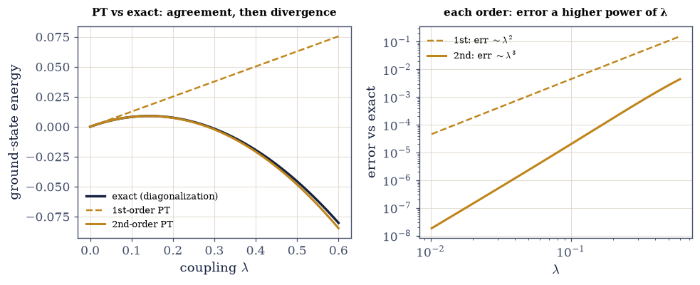
../../_images/64b752747751719116857a691ad1bba4f015553dfa88978495614bbfe4a4b056.png — Fig. 570 **Perturbation theory, watched holding and failing.** The ground-state energy of \(H_0+\lambda V\) as the coupling \(\lambda\) grows: the exact result from diagonalization (ink) against the first-order (dashed amber) and second-order (solid amber) perturbation series. At small \(\lambda\) all three coincide — the series is doing its job. As \(\lambda\) grows, first order (a straight line, the average of \(V\)) peels away first; second order, which curves downward with the level repulsion, follows the exact curve much further before it too departs. The error of the \(k\)-th order grows like \(\lambda^{k+1}\), so each order buys a wider window of validity, but none is exact away from \(\lambda=0\). This is the honesty a computer adds to perturbation theory: rather than trusting the expansion, we *see* precisely where ‘small correction’ stops being small — the inset shows the errors growing as powers of \(\lambda\).#

Exercise 3 — Where perturbation theory breaks#

Perturbation theory carries its own failure signal — the energy denominators. Here we close the gap between two levels and watch the second-order term blow up Eq. 610, Eq. 609.

Build two nearly-degenerate levels, \(E_0^0=0\) and \(E_1^0=\delta\) with \(\delta\) small, coupled by an off-diagonal \(V_{01}\).
Compute the second-order shift \(|V_{01}|^2/(E_0^0-E_1^0)\) and note it grows as \(1/\delta\).
Compare against the exact ground state (numpy.linalg.eigvalsh) as \(\delta\) shrinks, and show the overshoot growing.
Conclude that non-degenerate perturbation theory is invalid when levels approach — the cue for the degenerate treatment of Exercise 4.

two nearly-degenerate levels with a coupling — PT overshoots as the gap closes:
   gap δ     exact E₀     2nd-order PT     overshoot
  1.00     -0.00090     -0.00090      0.0000
  0.30     -0.00297     -0.00300      0.0000
  0.10     -0.00831     -0.00900      0.0007
  0.03     -0.01854     -0.03000      0.0115

Validation 3#

✓  the second-order shift overshoots the exact result for nearly-degenerate levels — PT fails when unperturbed levels are close (small denominators)

True

Exercise 4 — Degenerate perturbation theory as subspace diagonalization#

When the unperturbed level is degenerate the denominators vanish identically, and the fix is the most notorious piece of algebra in a quantum course — which on a computer is three lines: the “secular equation” is an eigh on a block, and the good basis is the one that diagonalizes \(V\) (§6.5) Eq. 611.

Write degenerate_pt(V, subspace_indices, states=None): restrict \(V\) to the listed states (columns of states, or the standard basis when states is None) and diagonalize that block with numpy.linalg.eigh Eq. 611, returning the first-order splittings (the eigenvalues) and the good states (the eigenvectors). Write this one yourself — the implementation is the lesson.
Build an \(H_0\) with a triply-degenerate level and a random Hermitian perturbation \(W\).
Restrict \(W\) to the degenerate subspace and diagonalize the block with it: the eigenvalues are the first-order splittings, the eigenvectors the good states.
Confirm the split levels \(E^0+\lambda\times(\text{splittings})\) match exact diagonalization of the full \(H\) (numpy.linalg.eigvalsh).

degenerate perturbation theory = eigh of V restricted to the degenerate subspace:
  first-order splittings (eigenvalues of V|subspace): [-1.3109 -0.0664  1.4561]
  degenerate-PT levels:  [0.97378 0.99867 1.02912]
  exact lowest three:    [0.97361 0.99865 1.02909]
  max error = 1.67e-04
the degeneracy is LIFTED; the eigenvectors are the 'good' zeroth-order states (§6.5)

Validation 4#

✓  degenerate PT is diagonalization of the perturbation within the degenerate subspace — matching exact to 1e-3   [max|Δ| = 0.000166755 (rtol=1e-06, atol=0.001)]

True

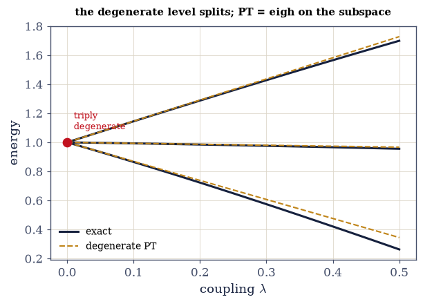
../../_images/9548ae49efc4b7ceeceeb2cb756ffb00c41fd274e7f51ba39aa3a90d9d18ee15.png — Fig. 571 **A degenerate level splitting.** A triply-degenerate unperturbed level (left, at \(E=1\)) as the perturbation is turned on (\(\lambda\) increasing to the right): the three exact eigenvalues (ink) fan out, and the degenerate-perturbation-theory prediction — \(E^0+\lambda\times\)(the eigenvalues of \(V\) restricted to the degenerate subspace) — tracks them (dashed amber) straight out of the degeneracy. This is the whole content of degenerate perturbation theory, which reads as forbidding algebra in a textbook: the ‘secular equation’ is nothing but `numpy.linalg.eigh` on the \(3\times3\) block of \(V\) within the degenerate subspace, and its eigenvectors are the ‘good’ states — the unique zeroth-order basis in which the perturbation is diagonal (the eigenspace projection of §6.5). Once the level has split, the pieces are non-degenerate and ordinary perturbation theory takes over. Hydrogen’s fine structure is exactly this problem, on the massively degenerate Coulomb levels.#

Exercise 5 — Hydrogen fine structure: the spin–orbit splitting#

The spin–orbit coupling \(H_{SO}\propto\mathbf L\cdot\mathbf S\) is the most famous ingredient of the fine structure, and it is a degenerate-perturbation problem whose good basis we already own: the coupled \(|j,m\rangle\) basis of §6.19, in which \(\mathbf L\cdot\mathbf S\) is diagonal Eq. 612.

Recall that in the coupled basis \(\mathbf L\cdot\mathbf S\) has eigenvalue \(\tfrac12[j(j+1)-l(l+1)-s(s+1)]\).
Build \(\mathbf L\cdot\mathbf S\) for \(l=1\), \(s=\tfrac12\) with the spin_orbit_operator helper (§6.19) and read off its distinct eigenvalues with numpy.linalg.eigvalsh.
Show \(j=\tfrac32\) is raised and \(j=\tfrac12\) lowered, and match the operator’s eigenvalues to the formula.
Identify the pattern as the sodium-D-type doublet.

spin–orbit L·S for l=1 (the good/coupled basis, 6.19):
  j=1.5 (2j+1=4):  ⟨L·S⟩ = +0.500   (raised; multiplicity 4)
  j=0.5 (2j+1=2):  ⟨L·S⟩ = -1.000   (lowered; multiplicity 2)
  L·S eigenvalues from the operator: [np.float64(0.5), np.float64(-1.0)]  (match the formula)
  trace check: tr(L·S) = +0.0e+00  (traceless, as required)
this doublet is the sodium D-line structure; spin–orbit lifts the degeneracy by j

Validation 5#

✓  the spin–orbit coupling splits levels by j (j=l+½ raised, j=l−½ lowered) with eigenvalue ½[j(j+1)−l(l+1)−¾]   [max|Δ| = 0 (rtol=1e-09, atol=1e-09)]

True

Exercise 6 — The full fine-structure formula and the lifted degeneracy#

Three relativistic corrections, all of order \(\alpha^2\), combine into one closed formula — and the punchline is which quantum numbers survive in it. The perfect Coulomb degeneracy of §6.17 is about to be lifted by relativity Eq. 612. The three corrections are the relativistic-kinetic term, the spin–orbit coupling, and the Darwin term; each is individually \(l\)-dependent, yet their sum collapses to \(E_{n,j}=-(\text{Ry}/n^2)[1+(\alpha^2/n^2)(n/(j+\tfrac12)-\tfrac34)]\) — quoted here rather than derived, as the conventions note above promised.

Write fine_structure_energy(n, j) returning that energy in eV, from the module constants RY and ALPHA.
Evaluate the \(n=2\) states: \(2S_{1/2}\), \(2P_{1/2}\), \(2P_{3/2}\).
Show \(2S_{1/2}\) and \(2P_{1/2}\) (same \(j=\tfrac12\), different \(l\)) coincide while \(2P_{3/2}\) splits off — the energy depends on \(j\), not \(l\): the \(l\)-degeneracy is lifted.
Compute the \(2P_{3/2}-2P_{1/2}\) splitting (\(\sim\alpha^2\text{Ry}\sim0.05\,\)meV) and note that its smallness is precisely what justifies perturbation theory.

hydrogen n=2 fine structure  Eₙⱼ = −(Ry/n²)[1 + (α²/n²)(n/(j+½) − ¾)]:
  2S₁/₂ (l=0,j=½):  E = -3.401480 eV
  2P₁/₂ (l=1,j=½):  E = -3.401480 eV
  2P₃/₂ (l=1,j=³⁄₂):  E = -3.401435 eV

  2S₁/₂ and 2P₁/₂ (same j=½) COINCIDE — energy depends on j, not l: the l-degeneracy is LIFTED by j
  2P₃/₂ − 2P₁/₂ splitting = 0.0453 meV  (scale α²Ry = 0.725 meV)
  tiny against 13.6 eV — which is exactly why perturbation theory is justified
  (a residual j=½ degeneracy remains, lifted by the Lamb shift — QED, a horizon)

Validation 6#

✓  the fine-structure energy depends only on n and j; the l-degeneracy of §6.17 is lifted (2P₃/₂−2P₁/₂ ≈ 0.045 meV)   [got 0.0452826 vs expected 0.0453 (rtol=1e-06, atol=0.005)]

True

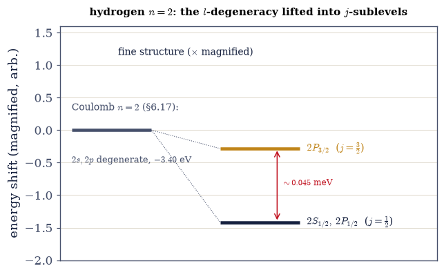
../../_images/25c5a473295fb491cd35cb3b26bb673cf2b9a46582a67201bdcb77d7ca3ab06f.png — Fig. 572 **Hydrogen’s fine structure: the \(l\)-degeneracy lifted.** The \(n=2\) level of hydrogen, hugely magnified. In the exact Coulomb problem of §6.17 (left) it is a single level at \(-3.40\,\)eV, holding the \(2s\) and \(2p\) orbitals at *precisely* the same energy — the \(l\)-degeneracy protected by the \(1/r\) potential’s hidden symmetry. Relativity breaks that symmetry: the three \(\alpha^2\) corrections (relativistic-kinetic, spin–orbit, Darwin) split the level (right, magnified \(\sim2.5\times10^4\times\)) into fine-structure sublevels labelled by the total angular momentum \(j\). The energy now depends only on \(n\) and \(j\), so \(2S_{1/2}\) and \(2P_{1/2}\) — same \(j=\tfrac12\), different \(l\) — remain degenerate, while \(2P_{3/2}\) (\(j=\tfrac32\)) lifts above them by \(\sim0.045\,\)meV. This tiny splitting is the fine structure of the Balmer lines and the archetype of the sodium D-line doublet; the residual \(2S_{1/2}\)–\(2P_{1/2}\) degeneracy is broken only by the Lamb shift of quantum electrodynamics.#

Exercise 7 — Perturbing the harmonic oscillator (student)#

The general method, turned on a familiar system: the anharmonic oscillator (§6.12), whose \(\lambda x^4\) correction admits no closed-form spectrum Eq. 608, Eq. 610.

Take the oscillator as \(H_0\) in the number basis (\(E_n=n+\tfrac12\) with \(\hbar=\omega=1\)).
Build \(x=(a+a^\dagger)/\sqrt2\) from the ladder operators and form the perturbation \(x^4\) with numpy.linalg.matrix_power.
Compute the first-order ground-state shift \(\lambda\langle0|x^4|0\rangle\).
Compare against exact diagonalization of \(H_0+\lambda x^4\) (numpy.linalg.eigvalsh) across \(\lambda\) and identify where perturbation theory breaks down.

anharmonic oscillator H = H₀ + λx⁴,  ⟨0|x⁴|0⟩ = 0.750:
   λ      exact E₀     1st-order PT (err)
  0.01   0.50726   0.50750 (2.4e-04)
  0.05   0.53264   0.53750 (4.9e-03)
  0.10   0.55915   0.57500 (1.6e-02)
  0.30   0.63799   0.72500 (8.7e-02)

  error at λ=0.01: 2.4e-04   error at λ=0.3: 8.7e-02  (grows with λ)

Validation 7#

✓  perturbation theory matches exact at small λ and diverges as λ grows for the λx⁴ anharmonic oscillator — its accuracy and breakdown, mapped

True

Exercise 8 — Approximation with a conscience (synthesis)#

Almost nothing in physics is exactly solvable, and perturbation theory is how we make progress anyway — by expanding around what we can solve and keeping the small terms. The formulas are simple: the average of the perturbation, then a sum over virtual transitions. But their honesty lives in the denominators: when two levels crowd together the expansion fails, and we must first find the good states by diagonalizing \(V\) within the degenerate subspace — degenerate perturbation theory, which on a computer is just a small eigh.

No new computation is left to do: the method, and its honesty, are the result. We did what no derivation can — watched the approximation agree with the exact answer and then part from it — and then turned it on the real prize: the fine structure that splits hydrogen’s degenerate levels by a few parts in a hundred thousand, lifting the \(l\)-degeneracy the Coulomb symmetry had protected (§6.17), through the spin–orbit coupling we posed in §6.18 and evaluated in §6.19. Movement V has begun. The next notebook (§6.22) turns to a different and often more powerful approximation — the variational method, which bounds the ground-state energy of systems too far from any solvable one for perturbation theory to reach, like the helium atom — and then the semiclassical WKB limit (§6.23) and time-dependent transitions (§6.24) complete the toolkit.

A good approximation knows its own limits. The virtue of doing perturbation theory on a computer is not that the computer does the algebra — it is that you can always ask the exact answer how well you did, and watch the honest place where “small correction” stops being small.

Notebook summary#

Perturbation theory, checked against exact — and hydrogen’s fine structure. The opening of Movement V.

First order Eq. 608: \(E_n^{(1)}=\langle n|V|n\rangle\), the average of the perturbation (numpy.vdot).
Second order Eq. 609: \(E_n^{(2)}=\sum_{m\ne n}|\langle m|V|n\rangle|^2/(E_n^0-E_m^0)\) — virtual transitions, level repulsion (\(E_0^{(2)}<0\)), and the energy denominators that decide validity.
Checked against exact Eq. 610: numpy.linalg.eigvalsh on \(H_0+\lambda V\) — agreement at small \(\lambda\), error \(\sim\lambda^{k+1}\), breakdown when levels are close.
Degenerate PT Eq. 611: numpy.linalg.eigh on \(V\) within the degenerate subspace — the splittings and the good states (the “secular equation,” §6.5), matching exact to \(10^{-3}\).
Fine structure Eq. 612: three \(\alpha^2\) corrections give \(E_{n,j}=-(\text{Ry}/n^2) [1+(\alpha^2/n^2)(n/(j+\tfrac12)-\tfrac34)]\) — the \(l\)-degeneracy of §6.17 lifted, split by \(j\) (\(2P_{3/2}\) above \(2P_{1/2}\) by \(\sim0.045\,\)meV), answering §6.18/§6.19.

We watched the approximation hold and fail against the exact answer, and used it to break hydrogen’s perfect degeneracy. Movement V is under way.

Outlook#

The variational method (§6.22): bounding ground-state energies from above, and the helium atom / a glimpse of variational Monte Carlo.
The WKB / semiclassical approximation (§6.23): and its connection to the Hamilton–Jacobi theory of Volume II (§2.10).
Time-dependent perturbation theory and Fermi’s golden rule (§6.24): transitions, selection rules, and spectra.
The Lamb shift and QED corrections beyond fine structure; hyperfine structure (horizons).
Cross-reference §6.5 (eigenspace projection / the good basis), §6.17 (the \(l\)-degeneracy), §6.18/§6.19 (spin–orbit, \(\mathbf L\cdot\mathbf S\)), §6.6 (compatible observables), and forward to §6.22, §6.23, §6.24.

Take this notebook with you

Use the download button (↓) in the toolbar above to save this notebook and run it yourself. The published notebooks ship without worked solutions; if you would like the reference solutions — to teach from or to check your own work — get in touch: hello@ramador.me.