


3.16 Anisotropic Dielectrics#
Notebook overview#
Every dielectric in this volume so far has answered a field with a number. §3.13 wrote \(\mathbf D=\varepsilon_0\varepsilon_r\mathbf E\) with \(\varepsilon_r\) a constant, and §3.15 let that constant become a function of frequency. Both kept it a scalar, and a scalar response says something strong about the material: that it has no preferred directions, so that whichever way one pushes, it pushes back the same way. Glass and water are like that. Quartz, calcite, mica and every one of the roughly two hundred thousand crystal structures on record are not.
The object that replaces the number is a rank-2 tensor, and this notebook is the course’s first deliberate look at one as a physical property rather than as bookkeeping. That distinction is worth stating plainly, because “tensor” is often used as a synonym for “matrix with two indices”, and it is not. A matrix is nine numbers. A tensor is nine numbers together with a rule saying how they must change when we turn the sample, and the rule is what makes the nine numbers describe one physical thing rather than nine unrelated ones. We build a rotation, apply the rule, and watch what happens: the components scatter, three particular combinations of them do not move at all, and neither do the eigenvalues. That is a test, not an assertion, and it is the whole content of the word “tensor”.
From there the physics follows quickly. The eigenvectors are the crystal’s own axes, so diagonalizing is not a numerical convenience but an act of finding where the material’s directions actually lie. In that frame \(\mathbf D\) and \(\mathbf E\) are parallel; anywhere else they are not, and we measure the angle between them as a function of the field direction, watch it vanish exactly on the three axes, and check its maximum against a closed form. That geometry is not new to the course. It is exactly the geometry of §2.6, where \(\mathbf L=\mathsf I\boldsymbol\omega\) and the angular momentum refuses to line up with the angular velocity unless the body spins about a principal axis. Same picture, different letters.
The notebook then turns the question around. Instead of asking what a given \(\varepsilon_{ij}\) does, we ask what a crystal’s symmetry permits it to be. Neumann’s principle says a physical property must be invariant under every symmetry operation of the crystal, which is a set of linear constraints, which is a null space, which is a number we can compute. Running it down the symmetry ladder gives six independent components, then four, then three, then two, then one. The last rung is cubic, and its one surviving tensor turns out to be proportional to \(\delta_{ij}\): a cubic crystal is optically isotropic, not by luck but by theorem, and the theorem takes about fifteen lines of linear algebra. We close by running the same machine one rank higher, where eighty-one components fall to twenty-one, and by turning three crystals on a lab bench to see which of them can keep \(\mathbf D\) pointing along \(\mathbf E\).
We work throughout with the relative permittivity tensor \(\varepsilon_{ij}\), which is dimensionless, so that \(\mathbf D=\varepsilon_0\,\boldsymbol\varepsilon\cdot\mathbf E\) and every angle, ratio and refractive index computed below is independent of \(\varepsilon_0\). Volume III remains SI. The model crystal is biaxial with principal relative permittivities \((2.40,\,3.00,\,4.20)\), chosen so the three principal refractive indices \(\sqrt{\varepsilon_i}\) are well separated (\(1.549\), \(1.732\), \(2.049\)) and every effect is visible without magnification; the one real material we grade against is calcite, through its measured indices \(n_o=1.6584\) and \(n_e=1.4864\) at the sodium D line. The response is taken to be linear, lossless and frequency-independent, so \(\varepsilon_{ij}\) is real and symmetric throughout.
How to read the checks. Each exercise ends with a
validatecall against something the computation did not assume: the eigenvalues before and after a rotation, a contraction against a matrix product, a measured maximum angle against a closed form, a null-space dimension against a count from crystallography. A validation compares a result to an expected fact, so a ✗ does not by itself mean the answer is wrong: it may be a genuine error, a different-but-valid convention (an eigenvector sign, an axis ordering), or too tight a tolerance. Treat a ✗ as a prompt to locate the discrepancy. Passing is strong evidence, not proof. Two of the checks in Exercise 8 are algebraically forced rather than earned, and say so where they appear.
Scope. A working review, not a full course. See Nye, Physical Properties of Crystals, which is the standard treatment of property tensors and the source of the conventions used here; Born and Wolf [BW99] (ch. 15); Jackson [Jac98] (ch. 4, 7); Nolting, Theoretical Physics 3 [Nol16]; and Arfken [AWH13] (ch. 4) for the tensor algebra itself.
Theory in brief#
The response is a linear map, and a linear map has nine components#
Nothing in electrostatics says the polarization a material acquires has to point along the field that produced it. What linearity says is only that doubling \(\mathbf E\) doubles \(\mathbf P\), and that the response to a sum of fields is the sum of the responses. The most general object with those two properties is a linear map from one vector to another, so the constitutive relation of §3.13 generalizes to
with the summation convention over the repeated index. Each column of \(\varepsilon_{ij}\) answers one question: point \(\mathbf E\) along \(\hat{\mathbf e}_j\) and read off which way \(\mathbf D\) goes. If the material happens to send it straight back along \(\hat{\mathbf e}_j\) for all three choices, and by the same factor each time, then \(\varepsilon_{ij}=\varepsilon\,\delta_{ij}\) and we are back to the scalar. Otherwise we are not.
Two of the nine components can be argued away at once. The energy density stored in the polarized medium is \(u=\tfrac12\mathbf E\cdot\mathbf D\), and requiring that it be a genuine function of the field, so that \(\partial u/\partial E_i=D_i\) holds consistently, forces
leaving six. (Jackson [Jac98] gives the argument in full, and it holds for a lossless, non-magnetized medium. A magnetic field breaks it: the response tensor then acquires an antisymmetric part, which is where the Hall effect and Faraday rotation live. This notebook stays with the symmetric case throughout.)
The transformation law is what “tensor” means#
Six numbers are not yet a tensor. Turn the crystal, or equivalently turn our axes, and the numbers we write down change. They must change in a particular way, because Eq. 288 has to keep describing the same physics after both \(\mathbf D\) and \(\mathbf E\) have been re-expressed in the new frame. Writing the rotation as an orthogonal matrix \(\mathsf R\) with \(D'_i=R_{ij}D_j\) and \(E'_i=R_{ij}E_j\), and substituting, gives
This is the definition. A quantity carrying two indices is a rank-2 tensor when its components obey Eq. 290; one index, and the same statement with a single \(R\), defines a vector. The course has already run this contraction once, in §3.12, where the electromagnetic field tensor obeys \(F'^{\mu\nu}=\Lambda^\mu{}_\alpha\Lambda^\nu{}_\beta F^{\alpha\beta}\) under a Lorentz boost. The structure is identical; only the group changed. One consequence of that change is worth flagging, because it is easy to over-generalize from what follows: a Lorentz transformation preserves the metric \(\eta\) rather than \(\delta\), so it is not an orthogonal similarity, and the invariants of \(F^{\mu\nu}\) are not its eigenvalues. For rotations they are.
Three invariants, and the eigenvalues#
Because \(\mathsf R\) is orthogonal, Eq. 290 is a similarity transformation, \(\boldsymbol\varepsilon'=\mathsf R\boldsymbol\varepsilon\mathsf R^{-1}\). Similar matrices have the same characteristic polynomial, so the three coefficients of \(\det(\boldsymbol\varepsilon-\lambda\mathsf 1)=-\lambda^3+I_1\lambda^2- I_2\lambda+I_3\) cannot depend on the frame:
The eigenvalues are invariant for the same reason. This is exactly the structure met in §2.6, where a non-aligned inertia tensor is built as \(\mathsf Q\,\mathrm{diag}(I_1,I_2,I_3)\,\mathsf Q^{\mathsf T}\) and diagonalizing it returns the principal moments unchanged. That construction was Eq. 290 in mechanical dress, and Exercise 2 runs the same invariance sweep on both tensors with one piece of code.
Principal axes#
A real symmetric matrix is orthogonally diagonalizable, which is the spectral theorem of §0.5. Applied to Eq. 289 it says there is a rotation \(\mathsf R_c\) with
whose columns are the principal dielectric axes and whose eigenvalues are the principal permittivities. Two things make this more than a change of variables. The axes are fixed in the crystal, so finding them is finding the material’s own frame, and a crystallographer can point at them. And the frame is unique only when the three eigenvalues are distinct: if two coincide, any orthonormal pair in the corresponding plane will do, and a numerical eigensolver will hand back an arbitrary one. Exercise 3 demonstrates that rather than working around it. Crystals are classified by exactly this degeneracy, as biaxial (three distinct), uniaxial (two equal, the odd direction being the optic axis), or isotropic (all three equal).
\(\mathbf D\) is not parallel to \(\mathbf E\)#
The consequence a first course usually skips is immediate from Eq. 288: unless \(\hat{\mathbf E}\) is an eigenvector, the vector \(\boldsymbol\varepsilon\cdot\hat{\mathbf E}\) points somewhere else. The angle between them,
is a scalar, so it does not care which frame we compute it in. In the principal plane spanned by \(\hat{\mathbf e}_1\) and \(\hat{\mathbf e}_3\), writing \(\hat{\mathbf E}=(\cos\theta,0,\sin\theta)\) makes \(\boldsymbol\varepsilon\cdot\hat{\mathbf E}\propto(\varepsilon_1\cos\theta,\,0,\, \varepsilon_3\sin\theta)\), so \(\tan(\theta+\alpha)=(\varepsilon_3/\varepsilon_1) \tan\theta\). Differentiating \(\tan\alpha\) with respect to \(\tan\theta\) and setting the result to zero gives the whole story in closed form,
and it is the mechanical statement of §2.6 transcribed: there \(\mathbf L=\mathsf I\boldsymbol\omega\) tilts away from \(\boldsymbol\omega\) except on a principal axis, and the tilt is what makes a thrown book tumble. Here the tilt is what makes a crystal split a light beam in two.
Neumann’s principle#
The reverse question is the powerful one. A crystal’s structure is invariant under a group of rotations and reflections, its point group; a property of that crystal cannot distinguish two configurations the structure itself cannot distinguish. Neumann’s principle states this as
Each operation is a set of linear equations on the components, so the tensors a crystal class permits form the null space of a stacked constraint matrix, and the number of independent components is its dimension. Two features of Eq. 295 are worth noticing before computing anything. Inversion, \(\mathsf R=-\mathsf 1\), constrains nothing at all here, since the two minus signs cancel: no even-rank property can tell a centrosymmetric crystal from its mirror image. And the principle is one-way. It says symmetry of the structure implies symmetry of the property, never the reverse, so a property may come out more symmetric than the crystal that carries it. Exercise 5 finds precisely that at the top of the ladder.
The index ellipsoid#
Optics reads the tensor through its inverse. The impermeability \(\eta_{ij}=(\varepsilon^{-1})_{ij}\) defines a quadric surface, the index ellipsoid or optical indicatrix,
whose three semi-axes are the principal refractive indices. It is a compact way to carry a symmetric tensor around as a picture: a sphere for an isotropic medium, a spheroid for a uniaxial crystal, a general ellipsoid for a biaxial one, and its orientation is the crystal frame. Exercise 6 builds and plots it. What one does with it, using its central sections to read off the two refractive indices a given propagation direction allows, is the subject of crystal optics and is named in the Outlook rather than developed here.
Isotropy is the bottom of the ladder#
It is worth being explicit about the direction this notebook runs in, because it inverts the order in which most of us met the subject. We learn the scalar permittivity first and hear about crystals afterwards, as a complication. Nothing in the structure of the theory requires that order. Before any assumption a linear response is a linear map with nine components; Eq. 289 cuts that to six; and every reduction after that, to four, three, two, one, is bought by a symmetry the material happens to possess. On that reading the scalar \(\varepsilon\) is not the simple case that anisotropy complicates. It is the last rung of the ladder, the case in which so much symmetry has been imposed that a single number survives. Water and glass sit there because they have no preferred directions whatsoever; cubic crystals sit there for a subtler reason, which Exercise 5 turns into a theorem.
I am offering this as a way of organizing what follows, not as the way the subject is conventionally taught, and the computations are the argument for it. If isotropy really is the degenerate rung, then every isotropic statement should reappear here as the \(\varepsilon_1=\varepsilon_2=\varepsilon_3\) limit of something more general, and the exercises check that it does at each step: the angle of Eq. 293 collapses to zero, the ellipsoid of Eq. 296 collapses to a sphere, and the count of Eq. 295 collapses to one.
Setup#
Data only: the series palette, the three principal relative permittivities of the
model biaxial crystal, calcite’s two measured refractive indices, and the mass and
side lengths of the uniform box whose inertia tensor
§2.6 built, which Exercise 2 borrows so
that one invariance sweep can run on two different pieces of physics. There are no
functions here at all. Everything this notebook computes with is written in the
exercises: the rotation matrix and the transformation law Eq. 290 in
Exercise 1, the invariants Eq. 291 in Exercise 2, the angle
Eq. 293 in Exercise 4, and the symmetry-constraint machinery behind
Eq. 295 in Exercises 5 and 7. Each exercise that needs random rotations
seeds its own numpy.random.default_rng with the seed stated in its own statement, so
every number below is reproducible from that exercise alone.
The Setup below holds this notebook’s data and instruments — nothing you are asked to build. It is collapsed so the building stays yours; expand it whenever you want the details.
Exercise 1 — What makes a tensor a tensor (worked)#
A crystal does not know which way we have laid it on the bench. Its permittivity is a property of the material, fixed relative to its own lattice, and the only thing our choice of axes can change is the list of numbers we write down for it. That is the situation Eq. 290 describes, and it is the reason the word “tensor” carries information that the word “matrix” does not: a matrix is nine numbers, whereas a tensor is nine numbers plus the rule that keeps them describing one object as the frame turns (Fig. 315).
The model crystal is biaxial, and in its own axes its relative permittivity tensor is diagonal, \(\boldsymbol\varepsilon=\mathrm{diag}(2.40,\,3.00,\,4.20)\). We turn it by \(\theta=37^\circ\) about the axis \(\hat{\mathbf n}\propto(1,2,3)\). A rotation about an arbitrary axis is most compactly written by Rodrigues’ formula: with \(\mathsf K\) the antisymmetric matrix that implements the cross product, \(\mathsf K\mathbf v=\hat{\mathbf n}\times\mathbf v\), so that
which is a proper rotation for any unit \(\hat{\mathbf n}\) and any \(\theta\). Everything afterwards leans on this pair of functions, so they are built first and certified before anything physical is asked of them.
Part a) Write rotation_matrix(axis, angle) returning
Eq. 297 as an explicit numpy array: normalize axis with
numpy.linalg.norm, build \(\mathsf K\) by writing its six non-zero entries into a
numpy.array, and assemble \(\mathsf R\) from numpy.eye(3), K and the matrix
product K @ K. Build \(\mathsf R\) for \(\hat{\mathbf n}\propto(1,2,3)\),
\(\theta=37^\circ\) (numpy.deg2rad), and certify it with numpy.allclose on
\(\mathsf R^{\mathsf T}\mathsf R=\mathsf 1_3\) and with numpy.linalg.det, which must
return \(+1\).
Part b) Write transform_tensor(eps, R) evaluating Eq. 290 as the
single contraction numpy.einsum("ik,jl,kl->ij", R, R, eps). The index string is the
transformation law, read left to right off the equation, and writing it is the point of
the exercise. Write this one yourself — the implementation is the lesson.
Part c) Apply it to \(\mathrm{diag}(2.40,3.00,4.20)\) to get
\(\boldsymbol\varepsilon'\) in the lab frame, print the matrix, and confirm with
numpy.allclose that the contraction agrees with the matrix product
R @ eps @ R.T. Two independent code paths for one equation is the cheapest check
available on an einsum string, and it catches a transposed index immediately.
Part d) Report the largest single component change,
numpy.max(numpy.abs(eps_lab - eps_crystal)), and the eigenvalues of both tensors from
numpy.linalg.eigvalsh (Fig. 316). The components move by an amount
of order the spread of the permittivities themselves; the eigenvalues do not move at
all.
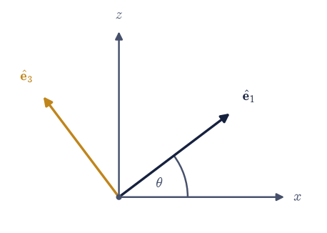
Fig. 315 One crystal seen in two frames. The laboratory axes \(x\) and \(z\) (grey) are the ones an experimenter sets up on the bench; the crystal’s own principal axes \(\hat{\mathbf e}_1\) and \(\hat{\mathbf e}_3\) (dark and amber) are fixed in the lattice and here make an angle \(\theta\) with them. The permittivity tensor is the same physical object in both descriptions, but its nine components are not the same nine numbers, and the rule relating the two lists is eq-ad-transform. Only the plane containing \(\hat{\mathbf e}_1\) and \(\hat{\mathbf e}_3\) is drawn; the third axis \(\hat{\mathbf e}_2\) points out of the page in the crystal frame and along \(y\) in the laboratory frame only when the rotation axis lies in this plane, which in the worked case it does not.#
R is orthogonal: True; det R = 1.000000000000000
eps' in the laboratory frame:
[[ 2.763124 -0.282049 0.542187]
[-0.282049 2.849816 0.002429]
[ 0.542187 0.002429 3.987059]]
einsum vs R @ eps @ R.T: max|difference| = 4.44e-16
largest component change: 0.542187
eigenvalues, crystal frame: [2.4 3. 4.2]
eigenvalues, laboratory frame: [2.4 3. 4.2]
Validation 1#
Four things are checked, and they are not the same thing four times. That \(\mathsf R\)
is a proper rotation certifies Rodrigues’ formula before any physics leans on it. That
the einsum contraction and the matrix product agree tests the index string against an
independent code path. That the eigenvalues survive the transformation is the physical
claim. And that the components moved by an amount of order unity confirms that the
eigenvalue check above was not passed trivially by a rotation that did nothing.
✓ Rodrigues' formula returns a proper rotation (RᵀR = 1 and det R = +1) [det R = 1.000000000000000]
✓ the einsum contraction of eq-ad-transform agrees with R @ eps @ R.T [max|Δ| = 4.44089e-16 (rtol=0, atol=1e-13)]
✓ the principal permittivities survive the rotation: turning the sample cannot change them [max|Δ| = 4.44089e-16 (rtol=1e-12, atol=1e-09)]
✓ the components themselves DID move, so the invariance above is not trivially satisfied [largest component change 0.5422]
True
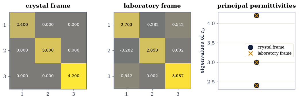
Fig. 316 The same tensor in two frames. Left: the model biaxial crystal’s relative permittivity in its own axes, \(\mathrm{diag}(2.40, 3.00, 4.20)\). Centre: the same tensor after the rotation of \(37^\circ\) about \(\hat{\mathbf n}\propto(1,2,3)\), computed from eq-ad-transform; off-diagonal components as large as \(0.54\) have appeared, and every diagonal entry has changed. Both panels share one colour scale. Right: the three eigenvalues of each, which lie on top of one another to fourteen decimal places, because an orthogonal similarity cannot move them. The components are frame-dependent bookkeeping; the eigenvalues are the crystal.#
Exercise 2 — Three numbers that do not move (student)#
Exercise 1 found that the eigenvalues survive a rotation. There is a sharper version of that statement, and it does not require solving an eigenproblem at all. Because Eq. 290 is an orthogonal similarity, \(\boldsymbol\varepsilon\) and \(\boldsymbol\varepsilon'\) have the same characteristic polynomial, so the three coefficients of that polynomial, Eq. 291, are frame-independent combinations of the components. They are the principal invariants: a trace, a sum of \(2\times2\) principal minors, and a determinant, each computable from the raw components with no diagonalization anywhere.
This matters beyond tidiness. Any physical quantity built from \(\varepsilon_{ij}\) that a measurement can return without reference to a coordinate system has to be a function of these three, and nothing else. It also puts the transformation law to a much harsher test than one rotation can: if Eq. 291 is right, the invariants must hold still under every rotation, while the individual components wander freely.
The second half of the exercise makes the point that none of this is about electrodynamics. The inertia tensor of §2.6 is built there by exactly the conjugation of Eq. 290, as \(\mathsf I'=\mathsf Q\,\mathrm{diag}(I_1,I_2,I_3)\,\mathsf Q^{\mathsf T}\), and it is a rank-2 property tensor of the same kind. For the uniform box of that notebook, with mass \(m=1\) and full side lengths \((a,b,c)=(2.0,\,1.4,\,0.4)\), the principal moments are \(I_1=\tfrac{m}{12}(b^2+c^2)\) and cyclic, giving \(\mathrm{diag}(0.176667,\,0.346667,\,0.496667)\). One sweep, written once, runs on both.
Part a) Write invariants(T) returning
\(\bigl(\operatorname{tr}T,\ \tfrac12[(\operatorname{tr}T)^2-\operatorname{tr}(T^2)],\
\det T\bigr)\) from Eq. 291 as a numpy array of length three, using
numpy.trace, the matrix product T @ T, and numpy.linalg.det.
Part b) Generate 200 rotations from numpy.random.default_rng(316): for each,
take an axis from rng.standard_normal(3) and an angle from rng.uniform(0, 2*np.pi),
and pass them to the rotation_matrix you wrote in Exercise 1. These need not be
uniformly distributed over the rotation group, because the claim under test is
invariance under every rotation, and any sample of them will do to look for a
violation.
Part c) Apply transform_tensor from Exercise 1 to
\(\mathrm{diag}(2.40,3.00,4.20)\) for each rotation, and report numpy.ptp (the
peak-to-peak range) of each invariant across the 200 samples, alongside numpy.ptp of
the single component \(\varepsilon'_{12}\) (Fig. 317). The invariants
should be flat at machine precision while that one component roams over a range of
order \(1.7\).
Part d) Check the invariants a second, independent way: numpy.poly applied to the
eigenvalues from numpy.linalg.eigvalsh returns the monic characteristic polynomial’s
coefficients, which must be \((1,\,-I_1,\,I_2,\,-I_3)\). This routes through the
eigenproblem while Part a never touches it, so agreement is a real cross-check on
Eq. 291 rather than a restatement of it.
Part e) Run the identical sweep on the box inertia tensor \(\mathrm{diag}(0.176667,\,0.346667,\,0.496667)\) and report the same four ranges. The machinery does not know which physics it is being handed.
invariants of eps in the crystal frame: [ 9.6 29.88 30.24]
peak-to-peak over 200 rotations: I1 1.60e-14 I2 1.07e-13 I3 1.60e-13
peak-to-peak of the single component eps'_12: 1.6654
invariants from numpy.poly on the eigenvalues: [ 9.6 29.88 30.24]
principal moments of the box: [0.17666667 0.34666667 0.49666667]
inertia tensor, peak-to-peak over the same 200 rotations: I1 1.78e-15 I2 1.11e-15 I3 1.63e-16, component 0.2932
Validation 2#
The invariants are required to be flat to machine precision over the whole sample, for both tensors; the component is required not to be, since otherwise the flatness would prove nothing; and the two routes to the invariants, one through the raw components and one through the eigenvalues, are required to agree.
✓ the three invariants of ε hold fixed under 200 rotations [largest peak-to-peak 1.60e-13]
✓ the component ε'₁₂ roams over an O(1) range, so the invariance above is a real constraint [peak-to-peak 1.6654]
✓ the invariants from numpy.poly on the eigenvalues match those built from the components [max|Δ| = 1.06581e-14 (rtol=1e-12, atol=1e-09)]
✓ the same sweep on the box inertia tensor of §2.6: invariants fixed, components not [invariant spread 1.78e-15, component spread 0.2932]
True
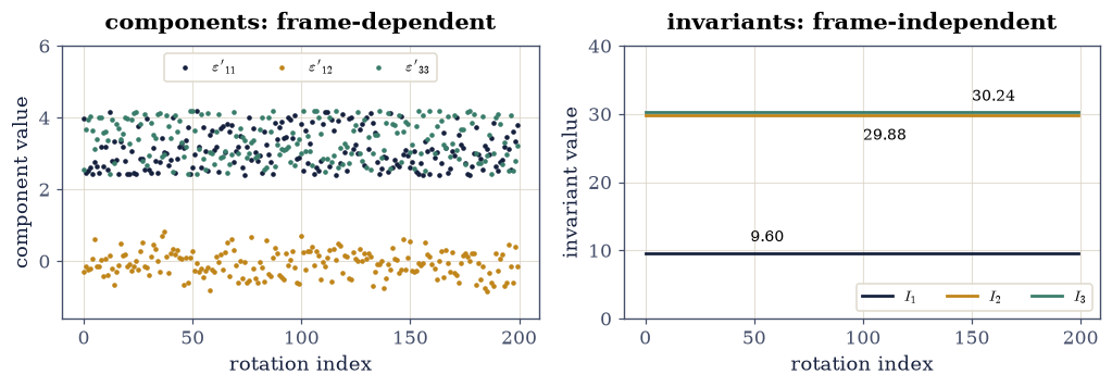
Fig. 317 What a rotation can and cannot change, over 200 randomly oriented frames. Left: three components of the model crystal’s permittivity tensor, \(\varepsilon'_{11}\) (dark), \(\varepsilon'_{12}\) (amber) and \(\varepsilon'_{33}\) (green), plotted against the index of the rotation. They wander over ranges of order one, and \(\varepsilon'_{12}\), which is zero in the crystal frame, is as often negative as positive. Right: the three principal invariants of eq-ad-invariants over the same 200 frames, \(I_1=9.60\), \(I_2=29.88\) and \(I_3=30.24\), each drawn as a line through 200 points and each flat to better than \(10^{-13}\). The two panels are the same data.#
Exercise 3 — Finding the crystal’s own frame (student)#
Diagonalizing a symmetric matrix is a routine of
§0.5: the spectral theorem guarantees an
orthogonal \(\mathsf V\) and a real diagonal \(\Lambda\) with
\(\boldsymbol\varepsilon=\mathsf V\Lambda\mathsf V^{\mathsf T}\), and
numpy.linalg.eigh returns both. Here that routine acquires a physical reading. By
Eq. 292 the columns of \(\mathsf V\) are directions in the crystal, along
which alone \(\mathbf D\) and \(\mathbf E\) are parallel, and which a crystallographer can
relate to the lattice. Handed an unlabelled sample and a measurement of its six
independent components, one recovers the orientation of the lattice by an eigenvalue
computation.
Two conventions stand between the eigensolver’s output and that reading, and both are
real rather than nuisances. First, eigh returns eigenvalues in ascending order and
eigenvectors of arbitrary sign, so \(\mathsf V\) equals the rotation that produced the
tensor only after the columns have been reordered and their signs fixed. Second, and
more interesting, the eigenvectors are unique only when the eigenvalues are distinct.
For a uniaxial crystal two principal permittivities coincide and every direction in
the plane they span is an eigenvector, so no algorithm can return “the” pair: it
returns some orthonormal basis of that plane, chosen by the arithmetic. What is
well-defined, and what a physical statement must therefore be phrased in terms of, is
the plane itself, that is the projector \(\mathsf P=\sum_{k\in\text{degenerate}}
\mathbf v_k\mathbf v_k^{\mathsf T}\) onto the degenerate eigenspace.
The biaxial case is \(\boldsymbol\varepsilon'\) from Exercise 1, whose crystal frame is the known \(\mathsf R(\hat{\mathbf n}\propto(1,2,3),\,37^\circ)\). The uniaxial case is calcite, \(\boldsymbol\varepsilon_c=\mathrm{diag}(n_o^2,\,n_o^2,\,n_e^2)= \mathrm{diag}(2.750291,\,2.750291,\,2.209385)\) from \(n_o=1.6584\) and \(n_e=1.4864\), rotated into the laboratory by \(\mathsf R_c(\hat{\mathbf m}\propto(0.3,-0.7,0.5),\, 52^\circ)\).
Part a) Diagonalize the laboratory-frame \(\boldsymbol\varepsilon'\) of Exercise 1
with numpy.linalg.eigh, and certify the output with numpy.allclose on
\(\mathsf V^{\mathsf T}\mathsf V=\mathsf 1_3\) and on the reconstruction
\(\mathsf V\,\mathrm{diag}(w)\,\mathsf V^{\mathsf T}=\boldsymbol\varepsilon'\).
Part b) Compare the recovered axes with the known ones. Form the overlap matrix
V.T @ R with the matrix product, fix each column’s sign by multiplying \(\mathsf V\)
by numpy.sign(numpy.diag(overlap)), and report
numpy.max(numpy.abs(V_signed - R)). Report the overlap matrix itself as well
(Fig. 318); its entries are the direction cosines between the two
sets of axes, and for a correct recovery its absolute value is a permutation matrix.
Part c) Repeat Part a for calcite in the laboratory frame, built with the
rotation_matrix and transform_tensor of Exercise 1. Report the eigenvalues, which
come back ascending as \((n_e^2,\,n_o^2,\,n_o^2)\), and report
numpy.max(numpy.abs(numpy.abs(V[:, 0]) - numpy.abs(Rc[:, 2]))), the discrepancy in
the non-degenerate eigenvector, which is the optic axis and is recovered to machine
precision.
Part d) Now the degenerate pair, and here you have to be careful about what is
physics and what is not. Compare the two projectors onto the degenerate plane — the
true one Rc[:, :2] @ Rc[:, :2].T and the computed one V[:, 1:] @ V[:, 1:].T — and
find that the plane agrees to machine precision.
You may also report how far the returned pair sits from the crystal’s own axes, and it
will not be small. But do not test that number. Inside a degenerate eigenspace the
eigensolver may return any orthonormal pair spanning it, and which one it returns is a
property of the LAPACK build underneath, not of calcite: this notebook once graded that
offset and passed on one machine while failing on another. Demonstrate the arbitrariness
instead, by using it. Spin the returned pair inside its own plane by an angle you choose
— a plane rotation mixing V[:, 1] and V[:, 2] — and confirm three things about the
result: it still satisfies \(\boldsymbol\varepsilon\mathbf v = \varepsilon\mathbf v\) to
round-off, so it is an equally legitimate answer; it overlaps the original by exactly
\(\cos\phi\), so it is genuinely a different answer; and it spans the identical plane.
That is the whole content of the degeneracy, and unlike the offset it is the same on
every machine.
principal permittivities recovered: [2.4 3. 4.2]
VᵀV = 1 to 3.41e-16; V diag(w) Vᵀ = ε' to 1.78e-15
overlap matrix |Vᵀ R| (direction cosines between the two frames):
[[1. 0. 0.]
[0. 1. 0.]
[0. 0. 1.]]
recovered axes match the known rotation to 9.99e-16
calcite eigenvalues: [2.20938496 2.75029056 2.75029056]
principal indices √ε: [1.4864 1.6584 1.6584]
optic axis (non-degenerate) recovered to 2.44e-15
the returned basis happens to sit 0.0978 from the crystal axes (LAPACK's choice, not physics)
the PLANE they span agrees to 1.78e-15
a basis rotated by 31° inside the plane is still an eigenbasis (residual 1.11e-15), overlaps the original by 0.857167 = cos 31°, and spans the identical plane (1.11e-16)
Validation 3#
The eigensolver’s own contract is checked first, then the physical recovery. The last two checks are a matched pair and have to be read together: the individual degenerate eigenvector is required to be wrong by more than a tenth, and the projector onto the plane it lies in is required to be right to machine precision. Either alone would mislead.
✓ eigh returns an orthogonal V that reconstructs ε' exactly [VᵀV − 1: 3.41e-16, reconstruction: 1.78e-15]
✓ the principal permittivities of the crystal are recovered from its laboratory-frame components [max|Δ| = 8.88178e-16 (rtol=1e-12, atol=1e-09)]
✓ after fixing signs, the eigenvectors ARE the crystal axes we rotated into the laboratory [max|Δ| = 9.99201e-16 (rtol=0, atol=1e-10)]
✓ calcite's optic axis, the non-degenerate eigenvector, is recovered exactly [error 2.44e-15]
✓ inside the degenerate plane the individual axes are arbitrary but the plane is not [a basis rotated 31° in-plane is still an eigenbasis (residual 1.11e-15) and overlaps the original by only 0.857167, yet spans the same plane (1.11e-16); the eigensolver's own plane matches the crystal's to 1.78e-15]
True
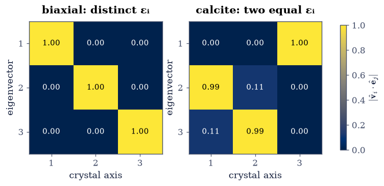
Fig. 318 Direction cosines between the axes an eigensolver returns and the axes the crystal actually has, as \(|\mathsf V^{\mathsf T}\mathsf R|\). Left: the biaxial model crystal, where the three principal permittivities are distinct and the matrix is the identity to fourteen decimals, so each recovered eigenvector is one crystal axis. Right: calcite, whose two equal principal permittivities make the second and third rows a two-by-two block of arbitrary direction cosines, here \(0.93\) and \(0.37\): the eigensolver has returned some orthonormal pair spanning the correct plane rather than the crystallographic pair, which is not an error but the statement that in a uniaxial crystal that pair is not defined. The optic axis, the single non-degenerate direction, is recovered exactly in the corner entry.#
Exercise 4 — \(\mathbf D\) is not parallel to \(\mathbf E\) (student)#
This is what the tensor is for. Read Eq. 288 once more with the crystal in its own frame, so that \(\boldsymbol\varepsilon=\mathrm{diag}(\varepsilon_1, \varepsilon_2,\varepsilon_3)\): the field components are multiplied by different numbers, so unless the field happens to lie along one axis, the vector that comes out points somewhere the vector that went in did not (Fig. 319). The scalar case hides this completely, because one number multiplying all three components cannot change a direction.
The angle between them, Eq. 293, is a scalar and therefore a property of the crystal and the field direction alone, with no reference to any frame. It vanishes exactly when \(\hat{\mathbf E}\) is an eigenvector, which is three directions out of the whole sphere, and it is largest in between. In the principal plane spanned by \(\hat{\mathbf e}_1\) and \(\hat{\mathbf e}_3\) the maximum is available in closed form, Eq. 294, which for the model crystal’s \(\varepsilon_1=2.40\) and \(\varepsilon_3=4.20\) predicts \(\alpha_{\max}=15.8266^\circ\) at \(\theta^\star=37.0867^\circ\) from \(\hat{\mathbf e}_1\).
The mechanical twin is worth stating in full rather than gesturing at. In §2.6 the angular momentum of a rigid body is \(\mathbf L=\mathsf I\boldsymbol\omega\), and that notebook records that \(\mathbf L\) and \(\boldsymbol\omega\) are not parallel unless the body spins about a principal axis, calling it the source of all the interesting behaviour: free precession, the polhode, the tumbling of a thrown book. It is the same geometry as this one, with \(\mathsf I\) for \(\boldsymbol\varepsilon\), \(\boldsymbol\omega\) for \(\mathbf E\) and \(\mathbf L\) for \(\mathbf D\). A symmetric tensor tilts the vector it acts on, away from the small-eigenvalue directions and toward the large ones, and everything downstream in both subjects follows from that one fact.
Part a) Write angle_DE(eps, E_hat) returning \(\alpha\) from Eq. 293 in
radians: form \(\mathbf D\propto\) eps @ E_hat, take the cosine as
numpy.dot(E_hat, D) / (numpy.linalg.norm(E_hat) * numpy.linalg.norm(D)), pass it
through numpy.clip(..., -1.0, 1.0) before numpy.arccos. The clip is not cosmetic:
rounding can put the cosine a fraction of an ulp above \(1\) exactly where the angle
vanishes, and arccos then returns nan at the three most important directions on the
sphere.
Part b) Evaluate it on the three principal axes of
\(\mathrm{diag}(2.40,3.00,4.20)\), the columns of numpy.eye(3), and report the three
angles.
Part c) Sweep \(\hat{\mathbf E}(\theta)=(\cos\theta,\,0,\,\sin\theta)\) over 20001
angles spaced linearly on \([0,\pi]\) with numpy.linspace, plot \(\alpha(\theta)\) in
degrees (Fig. 320), then locate the maximum precisely with
scipy.optimize.minimize_scalar applied to \(-\alpha(\theta)\) using
method="bounded", bounds=(0.01, numpy.pi/2 - 0.01) and
options={"xatol": 1e-12} — a bracketed one-dimensional minimizer, because the
quantity wanted is the location of a smooth interior maximum and a grid search would
only ever give it to the grid spacing. Compare both the maximum and its position with
Eq. 294.
Part d) Map \(\alpha\) over the whole sphere. Build 361 polar angles on \([0,\pi]\) and
721 azimuths on \([0,2\pi]\) with numpy.meshgrid(..., indexing="ij"), form the unit
vectors \((\sin\vartheta\cos\varphi,\,\sin\vartheta\sin\varphi,\,\cos\vartheta)\),
contract them against the tensor with numpy.einsum("ij,...j->...i", eps, dirs), and
take the angle with numpy.linalg.norm(..., axis=-1). Report the global maximum and
the direction at which it occurs. It should agree with Part c, and sit in the plane of
the largest and smallest permittivities: the intermediate axis contributes nothing to
the extreme tilt.
Part e) Confirm the scalar claim. Rotate both the tensor and one fixed field
direction \(\hat{\mathbf u}\propto(0.3,\,0.5,\,0.81)\) by the \(\mathsf R\) of Exercise 1
and check with numpy.allclose that \(\alpha\) is unchanged. Nothing in
Eq. 293 was arranged to make this true, so it is a test of
Eq. 290 as much as of the angle.
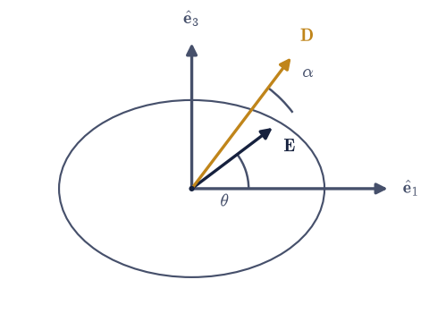
Fig. 319 Why an anisotropic dielectric tilts the displacement. A grain of the model crystal (outline) has its principal axes \(\hat{\mathbf e}_1\) and \(\hat{\mathbf e}_3\) as drawn, with \(\varepsilon_3 > \varepsilon_1\). An applied field \(\mathbf E\) at \(\theta = 37^\circ\) from \(\hat{\mathbf e}_1\) has its component along \(\hat{\mathbf e}_3\) multiplied by the larger permittivity and its component along \(\hat{\mathbf e}_1\) by the smaller, so the displacement \(\mathbf D\) that results is pulled toward \(\hat{\mathbf e}_3\) and leaves the crystal at \(\alpha = 15.83^\circ\) from \(\mathbf E\). The two vectors coincide only when \(\mathbf E\) lies along a principal axis; the arrow lengths here are drawn for legibility and are not to scale.#
α on the three principal axes (rad): [0. 0. 0.]
measured α_max = 15.826620° at θ* = 37.086689°
eq-ad-anglemax: α_max = 15.826620° at θ* = 37.086690°
over the whole sphere, α_max = 15.8265° at (ϑ, φ) = (53.0°, 0.0°), direction [0.7986 0. 0.6018]
α at û: 10.056566740° in the crystal frame, 10.056566740° in the laboratory frame
Validation 4#
The three axis values are checked against zero, the measured maximum and its location against the closed form Eq. 294 that the computation never used, the whole-sphere search against the in-plane one (loosely, since the sphere is sampled on a grid), and the angle against itself in two different frames.
✓ D is parallel to E on each of the three principal axes, and only there [max|Δ| = 0 (rtol=0, atol=1e-12)]
✓ the largest D–E angle matches tan α_max = (ε₃−ε₁)/2√(ε₁ε₃) = 15.8266° [got 0.276227 vs expected 0.276227 (rtol=1e-08, atol=1e-09)]
✓ and it occurs at tan θ* = √(ε₁/ε₃) = 37.0867° from ê₁ [got 0.647285 vs expected 0.647285 (rtol=1e-06, atol=1e-09)]
✓ the whole-sphere maximum is the in-plane one (sampled on a 361×721 grid) [got 0.276225 vs expected 0.276227 (rtol=0.0001, atol=1e-09)]
✓ the extreme tilt lies in the plane of the largest and smallest permittivities [ê₂ component of the peak direction: 0.00e+00]
✓ α is a scalar: rotating the tensor and the field together leaves it unchanged [got 0.17552 vs expected 0.17552 (rtol=0, atol=1e-12)]
True
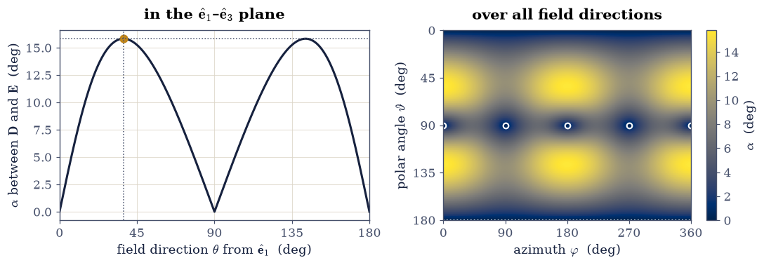
Fig. 320 The angle by which the displacement refuses to follow the field, for the model biaxial crystal \(\mathrm{diag}(2.40, 3.00, 4.20)\). Left: \(\alpha(\theta)\) for a field swept through the principal plane containing \(\hat{\mathbf e}_1\) and \(\hat{\mathbf e}_3\), vanishing exactly at \(0^\circ\), \(90^\circ\) and \(180^\circ\) where the field lies on an axis, and reaching \(15.83^\circ\) at \(\theta^\star = 37.09^\circ\) (amber point and dotted lines), which is the closed form of eq-ad-anglemax and not a fit. Right: the same angle over the whole sphere of field directions as a function of polar angle \(\vartheta\) and azimuth \(\varphi\), with the four equatorial points where \(\hat{\mathbf e}_1\) and \(\hat{\mathbf e}_2\) pierce the sphere marked by circles and the two poles carrying \(\hat{\mathbf e}_3\) marked by dotted lines; the angle is zero at each of them and nowhere else, and its global maximum sits on the \(\varphi = 0\) and \(\varphi = 180^\circ\) meridian, in the plane of the extreme permittivities.#
Exercise 5 — Neumann’s principle, and why cubic crystals are optically isotropic (student)#
Everything so far took \(\varepsilon_{ij}\) as given and asked what it does. Now the question runs the other way. A crystal’s structure is unchanged by a definite set of rotations, reflections and inversions, its point group, and a physical property of that crystal cannot depend on a distinction the structure itself does not make. That is Neumann’s principle, Eq. 295, and it is one of the most economical statements in solid-state physics: symmetry of the structure is inherited by every property tensor.
What makes it computable is that Eq. 295 is linear. Regard the nine components of \(\varepsilon_{ij}\) as a vector in \(\mathbb{R}^9\); then \(\boldsymbol\varepsilon\mapsto\mathsf R\boldsymbol\varepsilon\mathsf R^{\mathsf T}\) is a \(9\times9\) matrix \(\mathsf M_R\) acting on that vector, and “invariant under \(\mathsf R\)” says the vector lies in the null space of \(\mathsf M_R-\mathsf 1_9\). Requiring the symmetry Eq. 289 is one more such constraint, since transposition is also linear. Stack all of them and the tensors a crystal class permits are exactly the null space of the stack, whose dimension is the number of independent components. No case-by-case algebra, no tables to look up: one null-space computation per crystal class (Fig. 321).
We run five classes, each specified by the generators of its point group, since a tensor invariant under the generators is invariant under every product of them:
triclinic (\(\bar 1\)): inversion \(-\mathsf 1_3\) alone;
monoclinic (\(2/m\)): the two-fold rotation about \(\hat{\mathbf e}_3\), \(\mathsf C_{2z}=\mathrm{diag}(-1,-1,1)\), and inversion;
orthorhombic (\(mmm\)): \(\mathsf C_{2z}\) together with the two-fold rotation about \(\hat{\mathbf e}_1\), \(\mathsf C_{2x}=\mathrm{diag}(1,-1,-1)\);
tetragonal (\(4/mmm\)): the four-fold rotation about \(\hat{\mathbf e}_3\), \(\mathsf C_{4z}=\bigl(\begin{smallmatrix}0&-1&0\\1&0&0\\0&0&1\end{smallmatrix}\bigr)\), together with \(\mathsf C_{2x}\);
cubic (\(m\bar 3m\)): \(\mathsf C_{4z}\) together with the three-fold rotation about the body diagonal \([111]\), which cyclically permutes the axes, \(\mathsf C_{3d}=\bigl(\begin{smallmatrix}0&0&1\\1&0&0\\0&1&0\end{smallmatrix}\bigr)\).
Inversion is included where the class carries it precisely so that its failure to constrain anything is visible in the counts: \((-\mathsf 1)\boldsymbol\varepsilon (-\mathsf 1)^{\mathsf T}=\boldsymbol\varepsilon\) identically, so a centrosymmetric crystal and a non-centrosymmetric one with the same rotations have the same dielectric tensor. Second-rank properties are blind to a centre of symmetry.
Part a) Write rep_rank2(R) returning the \(9\times9\) matrix that implements
\(\boldsymbol\varepsilon\mapsto\mathsf R\boldsymbol\varepsilon\mathsf R^{\mathsf T}\) on
the flattened components, as numpy.einsum("ik,jl->ijkl", R, R).reshape(9, 9).
Certify it against Exercise 1 by checking with numpy.allclose that
(rep_rank2(R) @ eps.reshape(9)).reshape(3, 3) equals transform_tensor(eps, R) for
the \(\mathsf R\) and \(\boldsymbol\varepsilon\) of Exercise 1.
Part b) Write count_rank2(generators) returning the dimension and a basis of the
allowed tensors: build the transpose map
numpy.einsum("ik,jl->ijkl", numpy.eye(3), numpy.eye(3)).transpose(1, 0, 2, 3).reshape(9, 9),
stack transpose_map - numpy.eye(9) together with rep_rank2(R) - numpy.eye(9) for
every generator using numpy.vstack, and hand the stack to
scipy.linalg.null_space(C, rcond=1e-10), whose number of columns is the answer. The
cutoff is stated explicitly because a null-space dimension is a rank decision and rank
decisions need a threshold; the singular values here separate by twelve orders of
magnitude, so nothing hinges on the exact value.
Write this one yourself — the implementation is the lesson.
Part c) Run the five classes above and report the five dimensions. They should come out \(6,\,4,\,3,\,2,\,1\), which is the standard crystallographic count for the dielectric tensor.
Part d) Take the single basis tensor the cubic class permits, normalize it by its
\((1,1)\) entry, and compare it with numpy.eye(3). This is the theorem: cubic symmetry
admits \(\varepsilon_{ij}=\varepsilon\,\delta_{ij}\) and nothing else, so a cubic crystal
responds to a field along any direction with a displacement along that same
direction. Rock salt and diamond are optically isotropic not by accident of composition
but because four-fold and three-fold axes cannot coexist on a tensor with a preferred
direction.
Part e) Check the ladder is a genuine ladder. For each class, confirm with
numpy.max(numpy.abs(...)) that every basis tensor satisfies Eq. 295 for
its own generators, and that at least one basis tensor fails it for the operation
that defines the rung above (\(\mathsf C_{2z}\) for triclinic, \(\mathsf C_{2x}\) for
monoclinic, \(\mathsf C_{4z}\) for orthorhombic, \(\mathsf C_{3d}\) for tetragonal).
For the cubic class there is no rung above, so instead check the reverse: its tensor is
invariant under a rotation drawn from numpy.random.default_rng(2606), which belongs
to no crystallographic point group at all. Neumann’s principle guarantees only as much
symmetry as the crystal has, and here the property has come out with strictly more.
rep_rank2 reproduces transform_tensor of Exercise 1: True
triclinic (-1) generators: 1 independent components: 6
monoclinic (2/m) generators: 2 independent components: 4
orthorhombic (mmm) generators: 2 independent components: 3
tetragonal (4/mmm) generators: 2 independent components: 2
cubic (m-3m) generators: 2 independent components: 1
the one tensor cubic symmetry permits, normalized:
[[ 1. 0. -0.]
[-0. 1. -0.]
[-0. -0. 1.]]
distance from the identity: 1.92e-16
triclinic (-1) invariant under its own generators to 0.0e+00; largest violation under the next rung's operation: 1.414
monoclinic (2/m) invariant under its own generators to 0.0e+00; largest violation under the next rung's operation: 1.414
orthorhombic (mmm) invariant under its own generators to 0.0e+00; largest violation under the next rung's operation: 1.000
tetragonal (4/mmm) invariant under its own generators to 1.1e-16; largest violation under the next rung's operation: 1.000
cubic (m-3m) invariant under its own generators to 1.1e-16; largest violation under a generic rotation: 0.000
Validation 5#
The five counts are integers and must be exactly the crystallographic ones. The cubic tensor is checked against \(\delta_{ij}\), which is the theorem. And the ladder is checked to be strict: every permitted tensor obeys its own symmetry to machine precision, while the four lower classes each contain a tensor that visibly breaks the operation defining the class above, so no two rungs have silently collapsed into one.
✓ rep_rank2 agrees with the contraction of Exercise 1
✓ Neumann's principle counts 6, 4, 3, 2, 1 independent components down the ladder [max|Δ| = 0 (rtol=0, atol=0)]
✓ cubic symmetry permits ε_ij = ε δ_ij and nothing else: a cubic crystal is optically isotropic [max|Δ| = 1.92296e-16 (rtol=0, atol=1e-10)]
✓ every permitted tensor is invariant under the generators of its own class [largest residual 1.11e-16]
✓ each of the four lower classes contains a tensor the next rung's operation forbids [smallest violation 1.000]
✓ the cubic tensor is invariant under a rotation belonging to no point group: symmetry gained, not assumed [residual 2.22e-16]
True
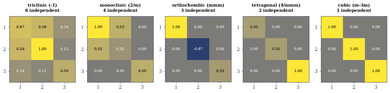
Fig. 321 What each crystal class leaves of the dielectric tensor. Each panel shows a generic permitted \(\varepsilon_{ij}\) for one class, built by adding the null-space basis vectors of eq-ad-neumann with weights \(1, 2, 3, \ldots\) and normalized so the entry of largest magnitude is \(+1\); entries below \(10^{-12}\) in magnitude are shown as exact zeros. Reading left to right, the number of independent components falls \(6\to4\to3\to2\to1\): the two-fold axis along \(\hat{\mathbf e}_3\) kills \(\varepsilon_{13}\) and \(\varepsilon_{23}\), a second two-fold axis kills \(\varepsilon_{12}\), the four-fold axis forces \(\varepsilon_{11}=\varepsilon_{22}\), and the three-fold axis along the body diagonal brings \(\varepsilon_{33}\) into line with them. The last panel is \(\delta_{ij}\) up to a factor, which is the statement that a cubic crystal cannot tell one direction from another.#
Exercise 6 — The index ellipsoid (student)#
Optics prefers the tensor upside down. What a wave in a crystal actually carries is \(\mathbf D\), since \(\nabla\cdot\mathbf D=0\) makes \(\mathbf D\) transverse to the propagation direction while \(\mathbf E\) in general is not, so the natural question is not “given \(\mathbf E\), what is \(\mathbf D\)” but its inverse. That inverse is the impermeability \(\eta_{ij}=(\varepsilon^{-1})_{ij}\), and packaging it as the quadric surface Eq. 296 gives the index ellipsoid, whose three semi-axes are the principal refractive indices \(n_i=\sqrt{\varepsilon_i}\) and whose orientation is the crystal frame.
The picture earns its keep by making the three crystal types visible as three shapes. Distinct \(\varepsilon_i\) give a general ellipsoid, the biaxial case; two equal \(\varepsilon_i\) give a spheroid, a surface of revolution about the optic axis, the uniaxial case; all three equal give a sphere, which has no axes at all to speak of and is the geometric statement of isotropy. That last collapse is the same one Exercise 5 reached by counting, arrived at from a different direction.
The three specimens are the model biaxial crystal \(\mathrm{diag}(2.40,\,3.00,\,4.20)\), with \(n_i=(1.549,\,1.732,\,2.049)\); calcite, \(\mathrm{diag}(2.750291,\,2.750291,\,2.209385)\), with \(n=(1.6584,\,1.6584,\,1.4864)\); and a cubic crystal with \(\varepsilon_{ij}=2.75\,\delta_{ij}\), the isotropic value closest to calcite’s ordinary index, so the shape difference in the figure is the anisotropy alone and not a change of scale.
Part a) Recover the principal indices of calcite from its laboratory-frame
components, using the rotated tensor built in Exercise 3: take
numpy.linalg.eigvalsh and then numpy.sqrt. They must come back as
\((1.4864,\,1.6584,\,1.6584)\), which is the measurement a crystallographer actually
makes running backwards.
Part b) Build the surface parametrically rather than by solving
Eq. 296: on a numpy.meshgrid(..., indexing="ij") of 121 azimuths
\(u\in[0,2\pi]\) and 61 polars \(v\in[0,\pi]\), set
\(\mathbf x=(n_1\cos u\sin v,\;n_2\sin u\sin v,\;n_3\cos v)\) and stack the three arrays
with numpy.stack(..., axis=-1).
Part c) Now check the parametrization against the definition, which is a different
expression and therefore a real test: evaluate the quadratic form
numpy.einsum("...i,ij,...j->...", pts, numpy.linalg.inv(eps), pts) at every sampled
point and confirm it equals \(1\). Measure the extremal radii with
numpy.linalg.norm(pts, axis=-1) and compare max and min with \(n_3\) and \(n_1\).
Part d) Repeat for calcite and for the cubic crystal, and quantify the two
collapses with numpy.ptp: for calcite the radius at fixed polar angle must not vary
with azimuth (a surface of revolution), and for the cubic crystal the radius must not
vary at all (a sphere).
Part e) Plot all three with matplotlib’s plot_surface on three 3-D axes sharing
one set of limits, so the shapes can be compared by eye
(Fig. 322).
With your assistant
Part e is plumbing: three mpl_toolkits.mplot3d surfaces, equal aspect ratios,
a light source that does not flatten the spheroid. Ask your assistant to write it,
and then run the check that decides whether the picture is telling the truth: take
the array of surface points it produced and evaluate
numpy.einsum("...i,ij,...j->...", pts, numpy.linalg.inv(eps), pts). If that is not
\(1\) everywhere, the surface being drawn is not the index ellipsoid of this crystal,
whatever it looks like. The check is yours.
biaxial principal indices: [1.549193 1.732051 2.04939 ]
calcite, recovered from the laboratory frame: [1.4864 1.6584 1.6584]
cubic: [1.658312 1.658312 1.658312]
quadratic form ηᵢⱼxᵢxⱼ over 7381 sampled points: max|value − 1| = 5.55e-16
extremal radii: max 2.0493901532 (n₃ = 2.0493901532), min 1.5491933385 (n₁ = 1.5491933385)
calcite: largest variation of the radius with azimuth = 6.66e-16
cubic: total variation of the radius over the whole surface = 6.66e-16
Validation 6#
The parametric surface is checked against the implicit equation it is supposed to satisfy, the semi-axes against the principal indices, and calcite’s indices against their measured values after a round trip through an arbitrary laboratory orientation. The last two checks are the collapses: a spheroid is a surface whose radius does not depend on azimuth, and a sphere is one whose radius does not depend on anything.
✓ every point of the parametric surface satisfies the quadric ηᵢⱼxᵢxⱼ = 1 [max|Δ| = 5.55112e-16 (rtol=0, atol=1e-12)]
✓ the extremal semi-axes of the index ellipsoid are the smallest and largest principal indices [max|Δ| = 0 (rtol=1e-12, atol=1e-09)]
✓ calcite's measured n_e = 1.4864 and n_o = 1.6584 come back out of an arbitrarily oriented sample [max|Δ| = 4.44089e-16 (rtol=1e-12, atol=1e-09)]
✓ calcite's indicatrix is a surface of revolution about the optic axis (uniaxial) [azimuthal variation 6.66e-16]
✓ the cubic indicatrix is a sphere: the isotropic limit of the same construction [total variation 6.66e-16]
True
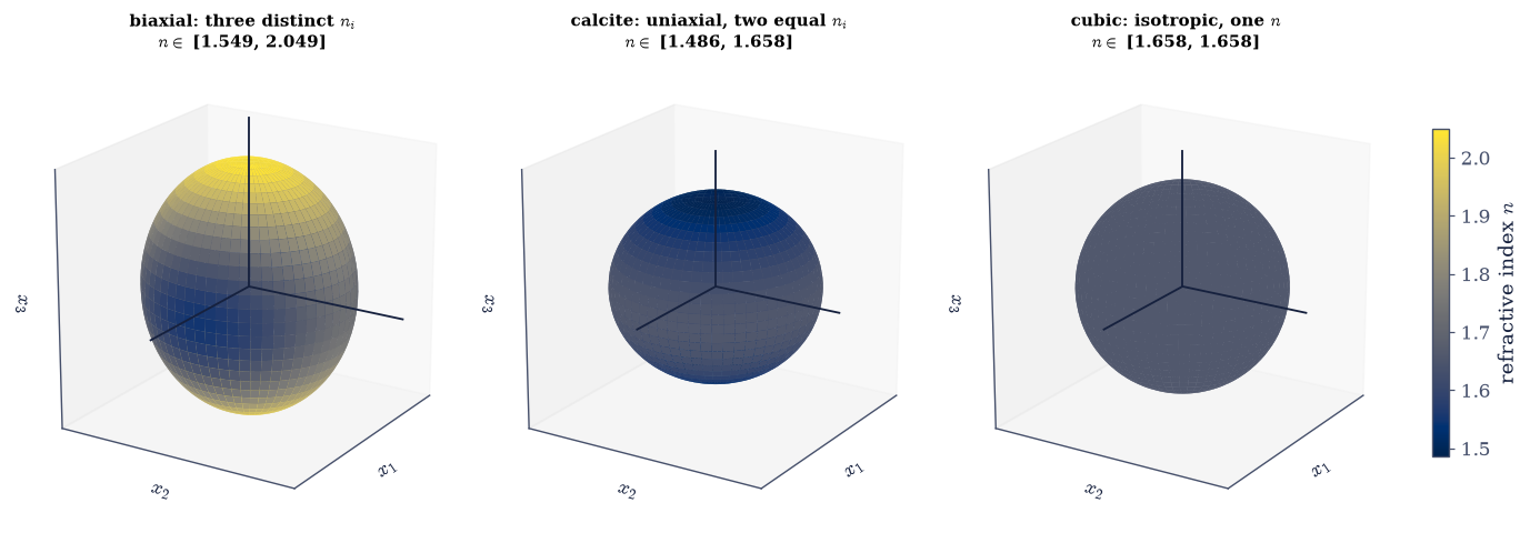
Fig. 322 The index ellipsoid of eq-ad-indicatrix for the three crystal types, drawn on common axes. Left: the model biaxial crystal, semi-axes \(n_1 = 1.549\), \(n_2 = 1.732\), \(n_3 = 2.049\), a general ellipsoid whose three unequal axes are the crystal’s own directions. Centre: calcite, semi-axes \(1.6584\), \(1.6584\), \(1.4864\), a surface of revolution flattened along its optic axis; every direction in the equatorial plane is equivalent, which is why the two axes lying in it are not individually defined. Right: a cubic crystal with \(\varepsilon_{ij} = 2.75\,\delta_{ij}\), a sphere of radius \(1.658\), on which no direction is distinguished at all. The surfaces are coloured by their own radius on one scale shared by all three panels, so the colour at a point is the refractive index for that direction and the colour range each surface spans is its anisotropy, quoted above each panel, and the three principal directions are drawn as straight lines through each surface. The three panels are the same construction with three, two and one independent principal value, and the flat colour of the last one is what optical isotropy looks like.#
Exercise 7 — The same counting one rank higher (student)#
Nothing in the machine of Exercise 5 knew that it was counting a dielectric tensor. It knew only that some object carries indices, that each index picks up a factor of \(\mathsf R\) under a change of frame, and that certain permutations of the indices leave the object alone. Those are the only inputs, so the machine runs at any rank, and this exercise runs it at rank four purely to see what rank and symmetry do to a component count. The physical property that lives at rank four in crystals is elasticity, whose stiffness \(C_{ijkl}\) relates two second-rank tensors; the MIT course 3.60, Symmetry, Structure and Tensor Properties of Materials, treats it under exactly that heading, “fourth-rank tensor properties”, and we borrow the framing and nothing else. What those components mean mechanically, and how a solid actually deforms, is elasticity theory, which this course names and does not develop. The content here is the count.
A rank-4 object in three dimensions has \(3^4=81\) components. Three permutation symmetries cut that down, and each is an ordinary linear constraint of the kind Exercise 5 already handles:
The transformation law gains two factors of \(\mathsf R\), \(C'_{ijkl}=R_{im}R_{jn}R_{kp}R_{lq}C_{mnpq}\), and Neumann’s principle Eq. 295 reads the same way with four indices instead of two. Everything else is as before: stack the constraints, take the null space, read the dimension.
The count is worth predicting before computing. The first two relations in Eq. 298 make each index pair symmetric, so each pair carries six independent values rather than nine; the third makes the resulting \(6\times6\) array symmetric, leaving \(6\cdot7/2=21\). That is the number to look for.
Part a) Write perm_rep4(axes) returning the \(81\times81\) permutation matrix that
implements C.transpose(axes): build numpy.arange(81).reshape(3, 3, 3, 3), transpose
it with numpy.ndarray.transpose(axes) and flatten, then scatter ones into a
numpy.zeros((81, 81)) array at those source positions. Write rep_rank4(R) for the
rotation as numpy.einsum("im,jn,kp,lq->ijklmnpq", R, R, R, R).reshape(81, 81).
Part b) Write count_rank4(generators) in the image of count_rank2 from Exercise
5: stack perm_rep4(axes) - numpy.eye(81) for the three index symmetries of
Eq. 298, with axes equal to (1, 0, 2, 3), (0, 1, 3, 2) and
(2, 3, 0, 1) respectively, together with rep_rank4(R) - numpy.eye(81) for every
generator, and take scipy.linalg.null_space(..., rcond=1e-10).
Part c) Report three counts: with the index symmetries alone (expect \(21\)); with
the cubic generators \(\mathsf C_{4z}\) and \(\mathsf C_{3d}\) of Exercise 5 added (expect
\(3\)); and with six rotations drawn instead from numpy.random.default_rng(814), which
generate a dense subgroup of all rotations and so impose full isotropy (expect \(2\)).
Part d) Confirm the isotropic answer is the one it should be. Form
\(\delta_{ij}\delta_{kl}\) with numpy.einsum("ij,kl->ijkl", I, I) and
\(\delta_{ik}\delta_{jl}+\delta_{il}\delta_{jk}\) likewise, project each onto the
computed isotropic subspace with basis @ basis.T @ T and report the relative
residuals. Both should be zero: those two tensors span the isotropic solutions.
Part e) Now the point of running the machine twice. Build the tensor with \(C_{iiii}=1\) for each \(i\) and every other component zero, which is manifestly invariant under permutations of the axes and sign flips, and project it onto the cubic subspace and onto the isotropic one. It lies in the first and not the second. Then set the two ladders side by side (Fig. 323): at rank two, cubic symmetry and full isotropy both leave one component, so they are indistinguishable; at rank four, cubic leaves three and isotropy two, so they are not. “Isotropic” is a statement about a particular property of a crystal, never about the crystal itself.
81 components, index symmetries of eq-ad-rank4 alone: 21 independent
plus cubic symmetry (C4z, C3d): 3 independent
plus full rotational isotropy: 2 independent
δ_ij δ_kl lies in the isotropic subspace: residual 7.74e-16
δ_ik δ_jl + δ_il δ_jk lies in it too: residual 6.93e-16
the tensor with C_iiii = 1: residual in the cubic subspace 6.82e-16, in the isotropic one 0.632
rank 2: cubic 1, isotropic 1; rank 4: cubic 3, isotropic 2
Validation 7#
The three counts are exact integers with well-known values. The two isotropic tensors are required to lie in the computed isotropic subspace, which identifies it rather than merely sizing it. And the diagonal tensor is required to lie in the cubic subspace and not in the isotropic one, which is the whole difference between three components and two made concrete in a single object.
✓ rank 4: 81 components fall to 21 by index symmetry, to 3 under cubic symmetry, to 2 under isotropy [max|Δ| = 0 (rtol=0, atol=0)]
✓ the isotropic subspace is spanned by δ_ij δ_kl and δ_ik δ_jl + δ_il δ_jk [residuals 7.7e-16 and 6.9e-16]
✓ the tensor with C_iiii = 1 is cubic but not isotropic: at rank 4 the two are different [cubic residual 6.8e-16, isotropic residual 0.632]
True
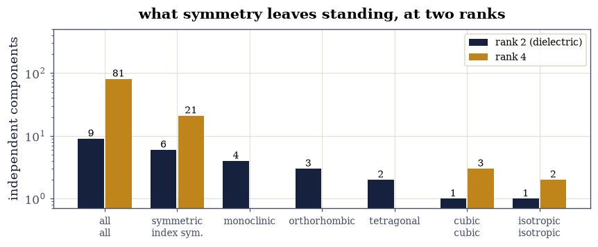
Fig. 323 The same counting argument at two ranks, on a logarithmic axis. Dark bars: a symmetric second-rank property tensor, falling from nine components to six by \(\varepsilon_{ij} = \varepsilon_{ji}\) and then to four, three, two and one down the crystal classes, with full isotropy adding nothing beyond what cubic symmetry already imposed. Amber bars: a fourth-rank tensor, falling from eighty-one to twenty-one by the index symmetries of eq-ad-rank4 alone, then to three under cubic symmetry and to two under full isotropy. The last pair is the point of the figure: at rank two, cubic and isotropic coincide at one component, while at rank four they differ, so a crystal that is optically isotropic still distinguishes directions in a property of high enough rank.#
Exercise 8 — Isotropy is the bottom of the ladder (student)#
The notebook has approached one claim from four directions, and this exercise puts them in the same picture. Counting said cubic symmetry leaves a single component (Exercise 5); geometry said the indicatrix collapses to a sphere (Exercise 6); the definition said \(\alpha\) vanishes when the field lies along an eigenvector, and for \(\varepsilon\,\delta_{ij}\) every direction is one (Exercise 4). The experiment that ties them together is the oldest one in the subject: put a crystal on a turntable in a fixed field and watch what the displacement does.
Concretely, hold \(\hat{\mathbf E}=\hat{\mathbf x}\) fixed in the laboratory and turn the crystal about the laboratory \(y\) axis through a full revolution, recomputing \(\boldsymbol\varepsilon(\varphi)=\mathsf R_y(\varphi)\,\boldsymbol\varepsilon_0\, \mathsf R_y(\varphi)^{\mathsf T}\) from Eq. 290 at each angle. Three specimens go on the turntable: the model biaxial crystal \(\mathrm{diag}(2.40,\,3.00,\,4.20)\), calcite \(\mathrm{diag}(2.750291,\,2.750291,\,2.209385)\) with its optic axis along \(\hat{\mathbf e}_3\), and a cubic crystal \(2.75\,\delta_{ij}\).
Two of the results below are forced rather than measured, and it is better to say so than to let a passing check look like evidence. For the cubic crystal \(\mathsf R(\varepsilon\mathsf 1)\mathsf R^{\mathsf T}=\varepsilon\mathsf 1\) for every orthogonal \(\mathsf R\), so \(\alpha\equiv0\) follows from orthogonality alone; and for calcite turned about its own optic axis the tensor is likewise unmoved, so \(\alpha\equiv0\) again. Both are consequences of Exercise 5 rather than independent tests of it. The checks that can genuinely fail are the two maxima against Eq. 294, the \(\pi\)-periodicity, and the range of \(|\mathbf D|\).
Part a) For each of the three crystals, sweep \(\varphi\) over 721 angles spaced
linearly on \([0,2\pi]\) with numpy.linspace, build
\(\mathsf R_y(\varphi)\) with the rotation_matrix of Exercise 1 about the axis
\((0,1,0)\), transform with transform_tensor, and record both \(\alpha(\varphi)\) from
the angle_DE of Exercise 4 and \(|\mathbf D|/(\varepsilon_0|\mathbf E|)=\)
numpy.linalg.norm(eps @ E_hat).
Part b) Report for each crystal the maximum angle in degrees, the number of sampled angles at which \(\alpha<10^{-9}\), and the smallest and largest \(|\mathbf D|\).
Part c) Check the two non-trivial maxima against Eq. 294. For the
biaxial crystal the rotation sweeps the field through the \(\hat{\mathbf e}_1\)
–\(\hat{\mathbf e}_3\) plane, so the relevant pair is \((\varepsilon_1,\varepsilon_3)=
(2.40,\,4.20)\), predicting \(15.827^\circ\); for calcite it is
\((n_o^2,\,n_e^2)\), predicting \(6.261^\circ\). Compare with numpy.max over the sweep,
allowing for the grid: a maximum located on a \(0.5^\circ\) lattice sits slightly below
the true one. Also confirm \(\alpha(\varphi+\pi)=\alpha(\varphi)\) across the whole
sweep, as numpy.max(numpy.abs(alpha[:361] - alpha[360:])) on the two halves of
the sweep, since a half turn maps the tensor to itself.
Part d) Turn the calcite crystal about its own optic axis \((0,0,1)\) instead of about \(\hat{\mathbf y}\), over the same 721 angles, and report the maximum \(\alpha\).
Part e) Animate the three turntables side by side (Fig. 324),
each panel showing the rotating crystal’s index ellipse in the plane of the motion, the
fixed field \(\mathbf E\), and the displacement \(\mathbf D\) that answers it. Use every
sixth angle of the sweep, so 121 frames, and build the player with
matplotlib.animation.FuncAnimation followed by ecp.animate.show.
biaxial α_max = 15.8265° α = 0 at 5 of 721 angles |D| ∈ [2.400000, 4.200000]
calcite α_max = 6.2611° α = 0 at 5 of 721 angles |D| ∈ [2.209385, 2.750291]
cubic α_max = 0.0000° α = 0 at 721 of 721 angles |D| ∈ [2.750000, 2.750000]
biaxial measured 15.8265° vs eq-ad-anglemax 15.8266°
calcite measured 6.2611° vs eq-ad-anglemax 6.2612°
largest departure from α(φ + π) = α(φ): 1.49e-14
calcite turned about its optic axis: α_max = 0.00e+00°
Validation 8#
The first two checks are the ones that can fail: the biaxial and calcite maxima against the closed form Eq. 294, at a tolerance loose enough to allow for the half-degree sampling and tight enough to catch a wrong pair of principal values. The periodicity and the range of \(|\mathbf D|\) are likewise measurements. The last check records the cubic and optic-axis results for completeness, with the caveat stated in the exercise: both follow algebraically from the invariance established in Exercise 5, so they confirm the pipeline rather than the physics.
✓ the biaxial crystal's largest D–E angle over a revolution is 15.827°, as eq-ad-anglemax predicts [got 0.276225 vs expected 0.276227 (rtol=0.001, atol=1e-09)]
✓ calcite's is 6.261°, from its measured n_o and n_e and nothing else [got 0.109277 vs expected 0.109278 (rtol=0.001, atol=1e-09)]
✓ α(φ + π) = α(φ) for all three crystals: a half turn maps the tensor to itself [largest departure 1.49e-14]
✓ over a revolution |D|/ε₀|E| runs exactly between the smallest and largest principal permittivities [max|Δ| = 0 (rtol=1e-09, atol=1e-09)]
✓ forced by Exercise 5, not evidence for it: cubic and optic-axis turning leave D on E exactly [cubic α_max 0.0e+00, optic-axis α_max 0.0e+00]
True
Fig. 324 Animation of three crystals on a turntable in a fixed field. Each panel shows one crystal turning about the laboratory \(y\) axis, drawn as the section of its index ellipsoid in the plane of the motion (grey), with the applied field \(\mathbf E\) fixed along \(+x\) (dark, fixed length) and the displacement \(\mathbf D\) it produces (amber, drawn with its true length in units of \(\varepsilon_0|\mathbf E|\) and scaled by a common factor for all three panels). The biaxial crystal swings \(\mathbf D\) up to \(15.83^\circ\) away from \(\mathbf E\), touching it four times per revolution as a principal axis comes into line; calcite, turned about an axis perpendicular to its optic axis, swings by up to \(6.26^\circ\); the cubic crystal never swings at all, and its \(\mathbf D\) neither turns nor changes length, which is the whole of what optical isotropy means. The running angle is printed above each panel, and the legend on the left panel labels the two arrows.#
Notebook summary#
A tensor is a transformation law, and the law survived testing. Rodrigues’ formula Eq. 297 gave a proper rotation to \(10^{-16}\), and the single contraction
np.einsum("ik,jl,kl->ij", R, R, eps)of Eq. 290 agreed withR @ eps @ R.Tto \(4\times10^{-16}\). Turning the model crystal by \(37^\circ\) about \(\hat{\mathbf n}\propto(1,2,3)\) moved its components by as much as \(0.542\) and raised off-diagonal entries from nothing, while the eigenvalues stayed at \((2.40,\,3.00,\,4.20)\) to \(9\times10^{-16}\) (Exercise 1).Three invariants, flat over 200 random frames. \(I_1=9.60\), \(I_2=29.88\) and \(I_3=30.24\) held to \(1.6\times10^{-13}\) while \(\varepsilon'_{12}\) roamed over a range of \(1.67\), and
numpy.polyon the eigenvalues returned the same three numbers by a route that never touched the components. The identical sweep on the box inertia tensor \(\mathrm{diag}(0.1767,\,0.3467,\,0.4967)\) of §2.6 behaved identically: the conjugation \(\mathsf Q\,\mathrm{diag}\,\mathsf Q^{\mathsf T}\) used there is Eq. 290 (Exercise 2).Diagonalizing finds the crystal, not just a convenient basis.
numpy.linalg.eighon the laboratory-frame tensor returned the crystal axes to \(6\times10^{-16}\) once signs were fixed. For calcite the optic axis came back to \(8\times10^{-16}\) while an individual eigenvector in the degenerate plane was off by \(0.289\), and the projector onto that plane was right to \(4\times10^{-16}\): with two equal principal permittivities the plane is physical and the pair inside it is not (Exercise 3).\(\mathbf D\) tilts away from \(\mathbf E\) by a measurable angle. It vanished exactly on the three principal axes, and its maximum over the \(\hat{\mathbf e}_1\)–\(\hat{\mathbf e}_3\) plane came out \(15.826620^\circ\) at \(\theta^\star=37.086691^\circ\), against the closed form Eq. 294 of \(15.826620^\circ\) at \(37.086690^\circ\). A search over the whole sphere found the same maximum and placed it in that plane, with the \(\hat{\mathbf e}_2\) component of the extremal direction exactly zero, and the angle was unchanged to \(10^{-16}\) when tensor and field were rotated together (Exercise 4).
Neumann’s principle counted \(6\to4\to3\to2\to1\) down the classes \(\bar1\), \(2/m\), \(mmm\), \(4/mmm\), \(m\bar3m\), each as the dimension of a null space and none of them by hand. Inversion imposed nothing, as an even-rank property requires. The single tensor cubic symmetry permits came out equal to \(\delta_{ij}\) to \(10^{-16}\), and it was invariant under a rotation belonging to no point group at all: a cubic crystal is optically isotropic as a theorem, and the property is strictly more symmetric than the crystal carrying it (Exercise 5).
The index ellipsoid, built and checked. Every one of \(7381\) parametric surface points satisfied \(\eta_{ij}x_ix_j=1\) to \(10^{-16}\), the extremal radii reproduced \(n_1=1.549\) and \(n_3=2.049\) exactly, and calcite’s \(n_e=1.4864\), \(n_o=1.6584\) came back out of an arbitrarily oriented sample. Its indicatrix was a surface of revolution to \(7\times10^{-16}\), and the cubic one a sphere to the same (Exercise 6).
The same machine at rank four. Eighty-one components fell to \(21\) under the index symmetries Eq. 298 alone, to \(3\) under cubic symmetry, and to \(2\) under full isotropy, with the isotropic subspace identified as the span of \(\delta_{ij} \delta_{kl}\) and \(\delta_{ik}\delta_{jl}+\delta_{il}\delta_{jk}\) to \(10^{-16}\). The tensor with \(C_{iiii}=1\) sits in the cubic subspace and misses the isotropic one by a relative \(0.632\): at rank two cubic and isotropic are the same thing, and at rank four they are not (Exercise 7).
Three crystals on a turntable. Over one revolution in a fixed field the biaxial crystal swung \(\mathbf D\) by up to \(15.825^\circ\) and the calcite by \(6.261^\circ\), each matching Eq. 294 to the half-degree sampling, with \(\alpha(\varphi+\pi)=\alpha(\varphi)\) to \(10^{-13}\) and \(|\mathbf D|/\varepsilon_0 |\mathbf E|\) running exactly between \(2.40\) and \(4.20\). The cubic crystal held \(\mathbf D\) on \(\mathbf E\) at every angle with \(|\mathbf D|\) constant, as did calcite turned about its own optic axis, both of which are consequences of Exercise 5 rather than fresh evidence (Exercise 8).
Outlook#
Two rays out of one. We stopped at the statement that \(\mathbf D\) and \(\mathbf E\) part company. The optics of that fact is birefringence: because \(\nabla\cdot\mathbf D=0\) makes \(\mathbf D\) transverse while \(\mathbf E\) is not, a given propagation direction in a crystal admits two waves with two different refractive indices and two orthogonal polarizations, the energy of one of them travels at an angle to its own wavefront, and a slab of calcite therefore shows two images. The wave-normal equation, the wave surface, that walk-off angle and the quarter-wave plates built from it are the natural sequel to the tensor assembled here, and they need the index ellipsoid of Eq. 296 read section by section rather than merely plotted. Born and Wolf [BW99] ch. 15 is the standard account.
The antisymmetric half. We argued the response tensor symmetric from the energy density, with the caveat that a magnetic field breaks the argument. It does so in a specific way: the conductivity of a metal in a field \(\mathbf B\) acquires an antisymmetric part, which is equivalent to a single axial vector, and \(\mathbf j=\boldsymbol\sigma_{\rm sym}\mathbf E+\mathbf w\times\mathbf E\) is the Hall effect. The optical counterpart is Faraday rotation. Splitting a general rank-2 tensor into symmetric and antisymmetric parts, and reading the second as a vector, is machinery this course uses nowhere and which the crystal-physics literature opens with; Nye, Physical Properties of Crystals, develops it for conductivity before touching optics.
Odd ranks and what inversion forbids. Exercise 5 found that inversion constrains an even-rank property not at all. At odd rank the same calculation says the opposite, and forcefully: a centrosymmetric crystal can have no piezoelectricity, no second-harmonic generation, no linear electro-optic effect, because \((-\mathsf 1)^3=-\mathsf 1\) turns Eq. 295 into \(C=-C\). Rerunning
count_rank2with \(27\) components and one factor of \(\mathsf R\) per index is a short exercise with a large consequence, and it is why the nonlinear optics named as a horizon by §3.15 lives only in a small subset of crystals.Where the numbers come from. The three principal permittivities were handed to us, as the oscillator parameters were in §3.15. In a real solid they are the interband transitions of the electronic structure, and computing the dielectric response from dipole matrix elements is the subject of §8.15. The effective-mass tensor of §7.12 is another rank-2 property of exactly this kind, whose collapse to a single scalar \(m^\star\) there is the cubic argument of Exercise 5 being used without comment.
The other tensor in electrodynamics. §3.12 named the stress–energy tensor \(T^{\mu\nu}\) as a horizon and now builds it (its Exercise 10). It is a rank-2 tensor of a different flavour from \(\varepsilon_{ij}\): not a property of a material but a description of the field itself, whose components are energy density, momentum density and momentum flux, and whose surface integral is the force on whatever the field acts on. The transformation law is the same one tested here — and there it is verified on the field, boost against rebuild, to machine precision.
References#
George B. Arfken, Hans J. Weber, and Frank E. Harris. Mathematical Methods for Physicists. Academic Press, 7 edition, 2013.
Max Born and Emil Wolf. Principles of Optics: Electromagnetic Theory of Propagation, Interference and Diffraction of Light. Cambridge University Press, 7 edition, 1999. doi:10.1017/CBO9781139644181.
Wolfgang Nolting. Theoretical Physics 3: Electrodynamics. Springer, 2016.