6.12 The Quantum Harmonic Oscillator

6.12 The Quantum Harmonic Oscillator#

    Elementary Computational Physics
  

Volume VI — Quantum Mechanics Notebook 6.12

The most important system in physics. Every potential near a minimum is a parabola, so the oscillator is the universal first approximation to almost everything — and it can be solved three ways that must agree: by an algebra of raising and lowering operators that produces the whole spectrum without a single derivative, by Hermite functions, and on the grid. We meet its zero-point energy, contrast it sharply with the classical oscillator, and build the coherent states that oscillate like a classical particle while staying as sharp as the uncertainty principle allows.

Level · advanced • Est. · 170–210 min

    Raymond Amador
    v1.4.0  ·  2026-07-31  · 
          CC BY 4.0 (text) / MIT (code)
  

Notebook overview#

If one had to pick a single system to understand deeply, it would be this one. The harmonic oscillator is the most important problem in physics, and for a reason that is almost embarrassingly simple: every smooth potential, near a stable minimum, is a parabola. Taylor-expand any well around its bottom and the leading term is \(\tfrac12V''(x_0)(x-x_0)^2\) — a harmonic oscillator. So the oscillator’s solution is the universal first approximation to vibrating molecules, the phonons of a crystal, and the modes of the electromagnetic field (each mode a quantum oscillator, its quantum the photon). Master it and you hold the leading description of an enormous swath of nature.

It earns a deep treatment because it can be solved three independent ways that must agree, and seeing them coincide is the structural lesson of the notebook. First, algebraically: from the single commutator \([a,a^{\dagger}]=1\), a pair of ladder operators generates the entire spectrum — equally-spaced levels \(E_n=\hbar\omega(n+\tfrac12)\) — with no differential equation at all. This is the Sakurai gem, and the same algebra returns for angular momentum (§6.14) and, in Volume VII, to count photons. Second, analytically: solving the differential equation gives the Hermite functions, whose ground state is exactly the minimum-uncertainty Gaussian of §6.9. Third, numerically: the §6.10 grid solver, reused. All three give the same spectrum and the same states.

Along the way we meet the features that make the quantum oscillator differ from Volume V’s classical one — a discrete, equally-spaced ladder and a nonzero zero-point energy \(\hbar\omega/2\) (it cannot sit at rest, forced by the uncertainty principle), against continuous energy and equipartition — and we watch the correspondence principle reconcile them at high quantum number. We finish with coherent states, the eigenstates of the lowering operator: the §6.9 Gaussian set in motion, which oscillate rigidly like a classical particle while staying minimum-uncertainty for all time — the cleanest bridge from quantum to classical motion, and the state of a laser field.

As in every Volume VI notebook, each exercise opens with a crystal-clear statement and enumerated parts, each naming the exact operation — the ladder matrices via numpy.diag with \(\sqrt n\) entries, numpy.linalg.eigh for the grid, numpy.polynomial.hermite.hermval for the Hermite polynomials, and math.factorial for the normalizations.

Two numerical notes. (i) numpy.math was removed in NumPy 2.0 — we use math.factorial (scipy.special.factorial is the array alternative), never np.math.factorial. (ii) The ladder matrices live in a truncated number basis of \(N_{\max}\) levels, so \([a,a^{\dagger}]=1\) holds only away from the top row and column (the truncation breaks it there); we verify it on the interior block and say so.

Conventions and scope. \(\hbar=m=\omega=1\), so \(E_n=n+\tfrac12\). The number basis is truncated at \(N_{\max}=40\); the grid solution uses the §6.10 finite-difference solver (eigenfunctions normalized by \(\sqrt{dx}\)). Squeezed states and the oscillator-as-photon are horizons (Volume VII). See Sakurai & Napolitano (§2.3, the operator method); Griffiths (the Hermite solution); and Notebooks §6.9 (the Gaussian, \([x,p]=i\hbar\)), §6.10 (the grid solver), §6.6 (uncertainty), and Volume V (the classical oscillator, equipartition).

Theory in brief#

Why the oscillator is everywhere#

Any smooth potential near a stable minimum is, by Taylor expansion, a parabola,

(554)#\[V(x)\approx\tfrac12 V''(x_0)\,(x-x_0)^2=\tfrac12 m\omega^2(x-x_0)^2,\qquad H=\frac{p^2}{2m}+\tfrac12 m\omega^2x^2 ,\]

so the oscillator is the universal leading description of molecules, phonons, and field modes.

The ladder operators — the algebraic solution#

The algebraic route begins with a factorization: up to an additive constant, \(H\) is a product of two first-order factors in \(x\) and \(p\). Define the lowering and raising operators

(555)#\[a=\sqrt{\tfrac{m\omega}{2\hbar}}\Big(x+\tfrac{ip}{m\omega}\Big),\quad [a,a^{\dagger}]=1,\quad H=\hbar\omega\big(a^{\dagger}a+\tfrac12\big)=\hbar\omega\big(N+\tfrac12\big),\quad N=a^{\dagger}a ,\]

with \(N\) the number operator. The entire spectrum follows from the algebra alone: \(a\) lowers the energy by \(\hbar\omega\) and \(a^{\dagger}\) raises it, the ground state obeys \(a|0\rangle=0\), and the ladder is \(a|n\rangle=\sqrt n\,|n-1\rangle\), \(a^{\dagger}|n\rangle=\sqrt{n+1}\,|n+1\rangle\), \(N|n\rangle =n|n\rangle\), giving \(E_n=\hbar\omega(n+\tfrac12)\) — equally spaced. (The same method returns for angular momentum, §6.14, and quantum fields.)

The zero-point energy#

The ladder bottoms out but the energy does not: the ground state is annihilated by \(a\), so \(N|0\rangle=0\), and the \(\tfrac12\) in \(H=\hbar\omega(N+\tfrac12)\) survives,

(556)#\[E_0=\tfrac12\hbar\omega\ne0 ,\]

the oscillator cannot sit at rest. This is the uncertainty principle (§6.6, §6.9): localizing the particle costs momentum spread, and minimizing \(\langle p^2\rangle/2m+\tfrac12 m\omega^2\langle x^2 \rangle\) subject to \(\Delta x\,\Delta p\ge\hbar/2\) gives exactly \(\hbar\omega/2\). (Zero-point energy is real — the Casimir effect, liquid helium; flagged, not developed.)

The analytic solution: Hermite functions#

Solving the differential equation directly, by the power-series method carried out in full in Griffiths, gives the Hermite functions,

(557)#\[\psi_n(x)=\Big(\tfrac{m\omega}{\pi\hbar}\Big)^{1/4}\frac{1}{\sqrt{2^n n!}}\,H_n(\xi)\,e^{-\xi^2/2},\qquad \xi=\sqrt{\tfrac{m\omega}{\hbar}}\,x ,\]

with \(H_n\) the Hermite polynomials (numpy.polynomial.hermite.hermval, math.factorial). The ground state is the Gaussian of §6.9 — the minimum-uncertainty state.

Three routes agree#

The three solutions arrive by entirely different means (commutators, a differential equation, a matrix), but they address one and the same eigenvalue problem, so their agreement is a theorem rather than a coincidence:

(558)#\[\{E_n,\psi_n\}_{\text{ladder algebra}}=\{E_n,\psi_n\}_{\text{Hermite}}=\{E_n,\psi_n\}_{\text{grid}} ,\]

the structural lesson: abstract algebra, special functions, and brute-force diagonalization are three views of one problem.

Classical versus quantum, and correspondence#

The quantum oscillator has discrete, equally-spaced levels and a nonzero ground-state energy; Volume V’s classical oscillator has continuous energy, obeys equipartition \(\langle E\rangle=kT\), and can rest at \(E=0\). They reconcile at high \(n\),

(559)#\[|\psi_n(x)|^2\ \xrightarrow{\ n\to\infty,\ \text{smoothed}\ }\ P_{\text{cl}}(x)=\frac{1}{\pi\sqrt{A^2-x^2}} ,\]

the classical distribution (a classical oscillator lingers near its turning points \(\pm A\), where it moves slowly): quantum mechanics contains classical mechanics in the large-\(n\) limit.

Coherent states — the most classical quantum state#

The eigenstates of the lowering operator,

(560)#\[a|\alpha\rangle=\alpha|\alpha\rangle,\qquad |\alpha\rangle=e^{-|\alpha|^2/2}\sum_n\frac{\alpha^n}{\sqrt{n!}}|n\rangle,\qquad \langle x\rangle(t)=\sqrt{\tfrac{2\hbar}{m\omega}}\,\mathrm{Re}\big(\alpha e^{-i\omega t}\big) ,\]

are coherent states — displaced ground states with \(\langle N\rangle=|\alpha|^2\). They are minimum-uncertainty (\(\Delta x\,\Delta p=\hbar/2\)) and stay so for all time, and they oscillate rigidly like a classical particle: the §6.9 Gaussian set in motion without spreading — the bridge from quantum to classical dynamics, and the state of a laser. Sakurai & Napolitano close §2.3 with their construction and properties.

Setup#

Data and instruments only: the units (\(\hbar=m=\omega=1\), so \(E_n=n+\tfrac12\)), the truncation \(N_{\max}=40\), the plotting colours, the §6.10 grid solver restated as a tool, and a one-line expectation value. The oscillator’s own machinery stays in your hands: you build the ladder operators in Exercise 1, the Hermite functions in Exercise 3, the number-basis \(x\) and \(p\) in Exercise 5, and the coherent state in Exercise 7.

The Setup below holds this notebook’s data and instruments — nothing you are asked to build. It is collapsed so the building stays yours; expand it whenever you want the details.

Exercise 1 — The ladder operators and the algebra#

Everything this notebook knows about the oscillator starts with one pair of matrices. In the truncated number basis \(\{|0\rangle,\dots,|N_{\max}-1\rangle\}\) the lowering operator carries \(\sqrt n\) on its upper off-diagonal, because \(a|n\rangle=\sqrt n\,|n-1\rangle\) shifts a state one rung down and weighs it by \(\sqrt n\); the raising operator is its transpose; and from the two come the number operator \(N=a^{\dagger}a=\mathrm{diag}(0,1,2,\dots)\) and the Hamiltonian \(H=\hbar\omega(N+\tfrac12)\) Eq. 555. Not a derivative anywhere — the algebra alone, no differential equation.

The defining relation is \([a,a^{\dagger}]=1\), and a truncated basis can honour it only away from the top: the missing \(|N_{\max}\rangle\) has nowhere to go, so the last row and column are spoiled and the identity holds on the interior block. That corner is worth looking at rather than hiding — it is the truncation making itself visible.

Write ladder_operators(n_max), returning \(a\), \(a^{\dagger}\), \(N\) and \(H\): \(a\) from numpy.diag(numpy.sqrt(numpy.arange(1, n_max)), 1), \(a^{\dagger}=a^{\mathsf T}\), \(N=a^{\dagger}a\), and \(H=\hbar\omega(N+\tfrac12)\). Write this one yourself — the implementation is the lesson.
Form the commutator \([a,a^{\dagger}]=aa^{\dagger}-a^{\dagger}a\) and confirm it equals the identity on the interior block.
Confirm \(N\) is \(\mathrm{diag}(0,1,2,\dots)\).
Print the bottom-right entry of the commutator, where the truncation shows.

[a,a†] = 1 on the interior block (away from truncation): True
  (the bottom-right corner is -39, not 1 — the truncation showing)
N = a†a = diag(0,1,2,…): True;  first few diagonal entries [0 1 2 3 4 5]

Validation 1#

✓  the ladder algebra [a,a†]=1 (away from the truncation) generates the number operator N=a†a=diag(0,1,2,…)

True

Exercise 2 — The spectrum from the algebra#

The spectrum is already in hand, and the argument for it is pure algebra: \(a|0\rangle=0\) defines the ground state, \(a^{\dagger}\) raises the energy by \(\hbar\omega\) and \(a\) lowers it, so the levels are the ladder \(E_n=\hbar\omega(n+\tfrac12)\), equally spaced Eq. 555. Because \(H\) is diagonal in the number basis, the energies can simply be read off its diagonal — no diagonalization, and no differential equation solved anywhere. This is the power that returns for angular momentum (§6.14) and, in Volume VII, for counting photons.

Read the energies off the diagonal of the \(H\) you built in Exercise 1.
Confirm they equal \(\hbar\omega(n+\tfrac12)\).
Confirm the level spacing is exactly \(\hbar\omega\).
Verify \(a|0\rangle=0\) on the basis vector \(|0\rangle\).

spectrum Eₙ from H: [0.5 1.5 2.5 3.5 4.5 5.5]
ℏω(n+½):            [0.5 1.5 2.5 3.5 4.5 5.5]   (match: True)
level spacing ΔE = 1.0000 = ℏω;  a|0⟩ = 0: True

Validation 2#

✓  the spectrum Eₙ = ℏω(n+½), equally spaced by ℏω, follows from the ladder algebra alone   [max|Δ| = 7.10543e-15 (rtol=1e-12, atol=1e-09)]

True

Exercise 3 — The grid solution agrees#

The third route is brute force: put the parabola \(V=\tfrac12 m\omega^2x^2\) on a box, hand the matrix to numpy.linalg.eigh through the §6.10 solve of the Setup, and see whether the numbers match the ladder Eq. 558. They must, and the comparison runs one way only: the algebraic spectrum \(\hbar\omega(n+\tfrac12)\) is exact, so every deviation the grid shows is discretization error. The highest levels converge last, their wave functions being wider and wigglier against a fixed grid — the §6.10 resolution caveat.

The analytic solution arrives here too, one exercise before it is examined, because the figure closing this exercise needs it: an eigensolver returns each eigenvector with an arbitrary global sign, and the states are drawn sign-aligned against their closed forms. That closed form is the Hermite function Eq. 557, \(\psi_n(x)=(m\omega/\pi\hbar)^{1/4}(2^n n!)^{-1/2}H_n(\xi) e^{-\xi^2/2}\) with \(\xi=\sqrt{m\omega/\hbar}\,x\). Evaluate \(H_n\) with numpy.polynomial.hermite.hermval, which takes a coefficient vector — a \(1\) in slot \(n\) and zeros elsewhere selects \(H_n\) — and take \(n!\) from math.factorial, cast to float so numpy.sqrt does not choke on a large Python integer. Exercise 4 grades the grid against it in earnest.

Write hermite_eigenfunction(n, x), returning \(\psi_n(x)\) as above.
Build \(V=\tfrac12 m\omega^2x^2\) on a box and solve with the §6.10 solve helper (numpy.linalg.eigh).
Compare the lowest six levels to \(\hbar\omega(n+\tfrac12)\).
Confirm the spacing is \(\hbar\omega\).

grid spectrum E[:6] = [0.5    1.5    2.4999 3.4998 4.4997 5.4995]
ℏω(n+½)             = [0.5 1.5 2.5 3.5 4.5 5.5]
max|E_grid − ℏω(n+½)| over the lowest 6 = 4.9e-04;  spacing ≈ 1.0000

Validation 3#

✓  the grid spectrum matches ℏω(n+½) with equal spacing ℏω — the algebra and diagonalization agree   [max|Δ| = 0.000489021 (rtol=1e-06, atol=0.001)]

True

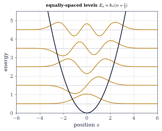
../../_images/037f03c4cea85986aacbded685edae415cbda65cad461599f32611de758ed1c2.png — Fig. 541 **The quantum harmonic oscillator.** The parabolic potential \(V=\tfrac12 m\omega^2x^2\) (ink) with its **equally-spaced** energy levels (dotted, \(E_n=\hbar\omega(n+\tfrac12)\)) and stationary states (amber) drawn at their energies. Two features distinguish it sharply from a classical oscillator: the levels are *discrete and uniformly spaced* by \(\hbar\omega\), and the lowest sits at \(\hbar\omega/2\) *above* the floor — a nonzero zero-point energy. The \(n\)-th state has \(n\) nodes and spreads wider as \(n\) grows, its bulk reaching toward the classical turning points. Every number here came from `numpy.linalg.eigh` on the grid, and it agrees to the digit with the ladder algebra and the Hermite functions.#

Exercise 4 — The eigenfunctions are Hermite functions#

Exercise 3 matched two spectra; the sterner test is the states themselves, function against function, point by point. The analytic answer is the Hermite function Eq. 557 — the hermite_eigenfunction you wrote in Exercise 3 — and the grid answer is a column of eigenvectors from numpy.linalg.eigh. Eigenvectors are defined only up to a global sign, so the comparison fixes the sign first by the overlap integral \(\int\psi_{\text{analytic}}\psi_{\text{grid}}\,dx\) and flips the numeric state when it comes out negative. What survives is discretization error, and it grows gently with \(n\) as the functions oscillate faster against a fixed grid — the same resolution story the energies told. The lowest state is worth naming: \(\psi_0(x)\propto e^{-m\omega x^2/2\hbar}\) is exactly the minimum-uncertainty Gaussian of §6.9, the second of the three routes closing on the first.

Evaluate \(\psi_n(x)\) on the Exercise 3 grid for \(n=0,1,2,3\) with your Exercise 3 hermite_eigenfunction.
Compare to the grid eigenfunctions from Exercise 3, flipping the sign so the overlap is positive.
Confirm agreement to within the grid’s discretization error.

max|ψ_grid − ψ_Hermite| for n=0,1,2,3: 7.34e-05  (grid discretization error)
the ground state ψ₀ ∝ e^(−mωx²/2ℏ) is the minimum-uncertainty Gaussian of §6.9

Validation 4#

✓  the eigenfunctions are the Hermite functions Hₙ(ξ)e^{−ξ²/2} (matching the grid)   [got 7.3405e-05 vs expected 0 (rtol=1e-06, atol=0.001)]

True

Exercise 5 — The zero-point energy#

The ladder bottoms out but the energy does not: \(E_0=\hbar\omega/2\ne0\), and the oscillator cannot be brought to rest Eq. 556. The reason is the uncertainty principle made energetic. Inverting the definitions of \(a\) and \(a^{\dagger}\) gives position and momentum back as \(x=\sqrt{\hbar/2m\omega}\,(a+a^{\dagger})\) and \(p=i\sqrt{\hbar m\omega/2}\,(a^{\dagger}-a)\), so both are available as matrices in the number basis you already have. In \(|0\rangle\) their means vanish, which makes \(\Delta x=\sqrt{\langle x^2\rangle}\) and \(\Delta p=\sqrt{\langle p^2\rangle}\), and minimizing \(\langle p^2\rangle/2m+\tfrac12 m\omega^2\langle x^2\rangle\) subject to \(\Delta x\,\Delta p\ge\hbar/2\) returns exactly \(\hbar\omega/2\): localizing the particle costs momentum spread, and the spread costs kinetic energy (§6.6, §6.9).

Build the number-basis \(x\) and \(p\) as X_OP and P_OP from the \(a,a^{\dagger}\) of Exercise 1.
Compute \(\langle x^2 \rangle\) and \(\langle p^2\rangle\) in \(|0\rangle\) (expval).
Form \(\langle H\rangle=\langle p^2 \rangle/2m+\tfrac12 m\omega^2\langle x^2\rangle\) and confirm it is \(\hbar\omega/2\).
Confirm \(\Delta x\,\Delta p=\hbar/2\) — the ground state saturates the bound.

⟨x²⟩ = 0.5000, ⟨p²⟩ = 0.5000
⟨H⟩ = ⟨p²⟩/2m + ½mω²⟨x²⟩ = 0.50000  (= ℏω/2 = 0.5)
Δx·Δp = 0.50000  (= ℏ/2 = 0.5: the ground state saturates the uncertainty bound)

Validation 5#

✓  the zero-point energy E₀=ℏω/2 is forced by the uncertainty principle (the ground state is minimum-uncertainty)   [max|Δ| = 1.11022e-16 (rtol=1e-06, atol=1e-09)]

True

Exercise 6 — Classical versus quantum, and the correspondence principle#

The two oscillators look nothing alike. The quantum one has discrete, equally-spaced levels and a ground state it cannot fall below; Volume V’s classical one has continuous energy, obeys equipartition \(\langle E\rangle=kT\), and rests at \(E=0\) when cold enough. They meet at high quantum number Eq. 559. A classical particle of energy \(E_n\) turns around at \(A=\sqrt{2E_n/m\omega^2}\) and moves slowest there, so it spends most of its period near the turning points and its dwell-time density is \(P_{\text{cl}}(x)=1/(\pi\sqrt{A^2-x^2})\) — the arcsine law, sharply peaked at \(\pm A\) and zero beyond them. The quantum density at large \(n\) oscillates far too fast to lie on that curve pointwise, but averaged over a few of its own wavelengths it is the same function: quantum mechanics contains classical mechanics as \(n\to\infty\), which is Bohr’s correspondence principle.

Tabulate the two side by side — levels, ground state, and statistics.
Compute the high-\(n\) density \(|\psi_n(x)|^2\) for \(n\approx30\) with your Exercise 3 hermite_eigenfunction.
Overlay the classical distribution \(P_{\text{cl}}(x)=1/(\pi\sqrt{A^2-x^2})\) with turning point \(A=\sqrt{2E_n/m\omega^2}\).
Smooth the quantum density with a running mean and confirm it tracks the classical envelope in the bulk.

                quantum oscillator        classical oscillator (Vol V)
  energies      discrete, ℏω-spaced       continuous
  ground state  E₀ = ℏω/2 ≠ 0             can rest at E = 0
  statistics    ─                          equipartition ⟨E⟩ = kT

high-n correspondence (n=30): smoothed |ψ|² vs classical 1/√(A²−x²), mean relative difference in the bulk = 0.10

Validation 6#

✓  the correspondence principle: the smoothed high-n |ψₙ|² approaches the classical distribution 1/√(A²−x²) — quantum becomes classical at large n

True

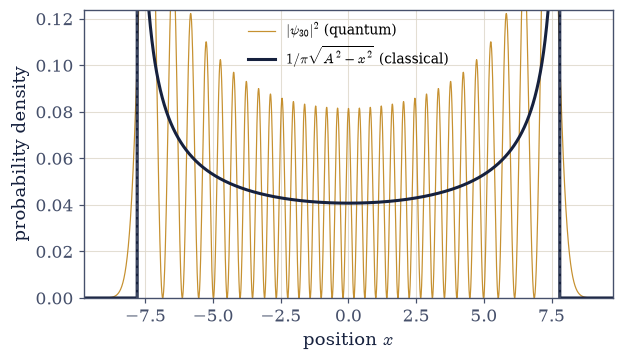
../../_images/7f260847510d7788d6436340f87e2e5a7a51a8dc8e67267e40cd43aac5f4a3c7.png — Fig. 542 **The correspondence principle.** The probability density \(|\psi_{30}(x)|^2\) of a high-lying oscillator state (amber) against the classical distribution \(P_{\text{cl}}(x)=1/(\pi\sqrt{A^2-x^2})\) (ink) for a classical particle of the same energy. The quantum density oscillates rapidly — \(n=30\) nodes — but its *envelope* tracks the classical one: both pile up near the turning points \(\pm A\), where a classical oscillator moves slowly and so spends most of its time, and both are cut off beyond them. Average the quantum wiggles over a few wavelengths and the two curves coincide. This is Bohr’s correspondence principle made visible: quantum mechanics *contains* classical mechanics in the limit of large quantum number.#

Exercise 7 — Coherent states#

The raising operator has no eigenstates worth the name, but the lowering operator has a whole family: the states with \(a|\alpha\rangle=\alpha|\alpha\rangle\), one for every complex \(\alpha\). Written in the number basis they are Poisson-weighted superpositions, \(|\alpha\rangle=e^{-|\alpha|^2/2}\sum_n(\alpha^n/\sqrt{n!})|n\rangle\) Eq. 560, with mean occupation \(\langle N\rangle=|\alpha|^2\). Two practicalities: \(n!\) comes from math.factorial cast to float, or numpy.sqrt overflows on the large Python integer; and the truncated basis cuts the \(n\ge N_{\max}\) tail, so the coefficients are renormalized and the eigenvalue test needs a tolerance rather than exact equality. Like the ground state, a coherent state saturates the uncertainty bound, \(\Delta x\,\Delta p=\hbar/2\) — it is the ground state, displaced — which makes it the most classical state the oscillator admits.

Write coherent_state(alpha, n_max), returning those normalized number-basis coefficients.
Verify it is an eigenstate of the lowering operator, \(a|\alpha\rangle=\alpha|\alpha\rangle\), with the \(a\) of Exercise 1 (numpy.allclose).
Confirm \(\langle N \rangle=|\alpha|^2\) (expval with the Exercise 1 number operator).
Compute \(\Delta x\,\Delta p\) with the X_OP, P_OP of Exercise 5 and confirm it is \(\hbar/2\).

a|α⟩ = α|α⟩ (eigenstate of the lowering operator): True
⟨N⟩ = 4.0000  (= |α|² = 4.0)
Δx·Δp = 0.50000  (= ℏ/2 = 0.5: minimum uncertainty — a displaced ground state)

Validation 7#

✓  a coherent state is a minimum-uncertainty eigenstate of the lowering operator (a|α⟩=α|α⟩, Δx·Δp=ℏ/2)   [max|Δ| = 1.04188e-12 (rtol=1e-06, atol=0.001)]

True

Exercise 8 — Coherent-state dynamics: a quantum particle that moves classically (student)#

Time evolution costs nothing in the number basis, because \(H\) is diagonal there: each component of a state simply acquires a phase, \(|\psi(t)\rangle=\sum_n c_n e^{-iE_nt/\hbar}|n\rangle\) (equivalently, and more expensively, scipy.linalg.expm(-1j*H*t) @ psi). Do that to the coherent state of Exercise 7 and something remarkable happens: its center traces the classical trajectory \(\langle x\rangle(t)=\sqrt{2\hbar/m\omega}\,\alpha\cos\omega t\) exactly, and its width never changes — \(\Delta x\,\Delta p=\hbar/2\) holds for every \(t\), not just at \(t=0\) Eq. 560. The rigidity is peculiar to the oscillator, whose equally-spaced levels keep every phase in step; a free particle’s packet spreads instead (§6.13). This is the bridge from quantum to classical motion, and the state of a laser field.

Evolve the \(|\alpha\rangle\) of Exercise 7 by phasing each number-basis component with \(e^{-iE_nt/\hbar}\), over one period.
Compute \(\langle x\rangle(t)\) with expval and the Exercise 5 X_OP.
Confirm it equals the classical trajectory \(\sqrt{2\hbar/m\omega}\,\alpha\cos\omega t\).
Confirm \(\Delta x\, \Delta p=\hbar/2\) is maintained for all \(t\).

⟨x⟩(t) quantum:   [ 2.828  2.449  1.414 -0.    -1.414 -2.449 -2.828]
classical cos:    [ 2.828  2.449  1.414  0.    -1.414 -2.449 -2.828]   (match: True)
Δx·Δp maintained at ℏ/2 for all t: True  (the packet does not spread — unique to the oscillator)

Validation 8#

✓  a coherent state oscillates like a classical particle, ⟨x⟩(t)=√(2ℏ/mω)α cos ωt, and stays minimum-uncertainty for all t   [max|Δ| = 1.55431e-15 (rtol=1e-06, atol=0.01)]

True

Fig. 543 **A quantum particle that moves classically, animated.** The probability density \(|\psi_\alpha(x,t)|^2\) of a coherent state (amber) sliding back and forth in the parabolic well (ink) — a Gaussian wave packet whose center traces the classical trajectory \(\langle x\rangle(t)=\sqrt{2\hbar/m\omega}\,\alpha\cos\omega t\) exactly, while its shape never changes. Of all quantum states this is the most classical: it is the minimum-uncertainty Gaussian of §6.9 set in motion, and it stays minimum-uncertainty for all time, neither spreading nor distorting. This rigidity is special to the harmonic oscillator (a free wave packet spreads, §6.13); it is why a coherent state describes the field of a laser, the closest a quantum system comes to a classical oscillating amplitude.#

Exercise 9 — The universal oscillator (synthesis)#

The harmonic oscillator is the system all of physics reduces to near a minimum, and we solved it three ways that had to agree — by an algebra that produced the entire equally-spaced ladder from the single commutator \([a,a^{\dagger}]=1\), by Hermite functions, and on the grid. Its zero-point energy \(\hbar\omega/2\) is the uncertainty principle made energetic; its high states recover the classical motion through the correspondence principle; and its coherent states oscillate like a classical particle while staying as sharp as quantum mechanics permits. The ladder operators built here are not a trick for one problem — they return for angular momentum (§6.14), and in Volume VII they will count photons.

There is no new computation to do here: the convergence of the three routes is the result. Of all the systems in this volume, this is the one met most often — in every molecule’s vibrations, every solid’s heat capacity, every mode of light. It is worth knowing three ways, because each is the natural language in a different setting: the algebra for fields and angular momentum, the Hermite functions for analytic work, the grid for any potential that is only approximately harmonic. The next notebook (§6.13) sets wave packets in motion through barriers, where — unlike the rigid coherent state — they spread and tunnel.

Notebook summary#

The oscillator solved three ways, with its zero-point energy, classical limit, and coherent states.

The ladder algebra Eq. 555: \(a,a^{\dagger}\) via numpy.diag (\(\sqrt n\) off-diagonal), \([a,a^{\dagger}]=1\) (away from truncation), \(N=a^{\dagger}a\) — the spectrum \(E_n=\hbar\omega(n+\tfrac 12)\) from the algebra alone.
Three routes agree Eq. 558: ladder, Hermite functions (numpy.polynomial.hermite.hermval, math.factorial), and the §6.10 grid (numpy.linalg.eigh) give the same spectrum and states.
Zero-point energy Eq. 556: \(E_0=\hbar\omega/2\), the ground state minimum-uncertainty — the uncertainty principle made energetic.
Correspondence Eq. 559: the quantum oscillator (discrete, zero-point) differs from Volume V’s classical one (continuous, equipartition), but the smoothed high-\(n\) density approaches the classical \(1/\sqrt{A^2-x^2}\).
Coherent states Eq. 560: \(a|\alpha\rangle=\alpha|\alpha\rangle\), minimum-uncertainty, oscillating rigidly as \(\langle x\rangle(t)=\sqrt{2\hbar/m\omega}\,\alpha\cos\omega t\) without spreading — the bridge to classical motion.

Every potential near a minimum is this one, and it is worth knowing all three ways — algebra, Hermite functions, and the grid.

Outlook#

The same ladder algebra for angular momentum (§6.14) and, in Volume VII, for photons and quantum fields.
Wave-packet dynamics, spreading, and tunnelling (§6.13) — the contrast to the non-spreading coherent state.
The oscillator as the photon: quantized field modes, the Casimir effect, the laser (Volume VII; horizons). Squeezed states (a horizon, named).
Cross-reference §6.9 (the Gaussian, uncertainty, \([x,p]=i\hbar\)), §6.10 (the grid solver), §6.6 (uncertainty), Volume V (the classical oscillator, equipartition), and forward to §6.13, §6.14, Volume VII.

Take this notebook with you

Use the download button (↓) in the toolbar above to save this notebook and run it yourself. The published notebooks ship without worked solutions; if you would like the reference solutions — to teach from or to check your own work — get in touch: hello@ramador.me.