7.10 The Fermi Gas at Finite Temperature: Sommerfeld’s 0.4%, and Two Mysteries Dissolved

Elementary Computational Physics

Volume VII — Quantum Statistical Mechanics Notebook 7.10

A metal's electrons live at effectively absolute zero; this notebook computes the 'effectively' — and finds two of the oldest puzzles of metal physics hiding in it. Why do the electrons show almost no heat capacity? Why are metals such feeble, temperature-blind paramagnets? One sentence answers both: Pauli blocks the bulk, and only the sliver of electrons within kT of the Fermi surface may respond. We make the sentence exact, read the Sommerfeld coefficient off the experimenter's plot, and follow the gas across two decades of temperature until it forgets it was ever quantum.

Level · advanced   •   Est. · 190–230 min

Raymond Amador v1.4.0  ·  2026-07-31  ·  CC BY 4.0 (text) / MIT (code)

Notebook overview

§7.9 established that a metal is, to its electrons, a system at absolute zero to within parts in a thousand. This notebook computes the parts in a thousand — and finds that they were, historically, two of the deepest puzzles in the physics of metals. The tool is the Sommerfeld expansion of §7.3, deployed at last on the integrals it was built for, and the physics is one sentence spoken twice: Pauli blocks the bulk; only the surface fraction \(\sim T/T_F\) participates.

The program runs on the chemical potential. Fixed particle number pins \(\mu(T)\) through the Fermi–Dirac integral, which we solve exactly (a root find at every temperature) and check against Sommerfeld’s \(\mu = \varepsilon_F[1 - (\pi^2/12)(T/T_F)^2]\) to six digits — at room temperature in copper, the sea’s level has moved by ten parts per million. Then the exact curve goes where the expansion cannot: \(\mu\) falls, crosses zero near \(T \sim T_F\), and lands on the classical asymptote \(k_BT\ln(n\lambda^3)\) of §7.8 — one function spanning both worlds.

The heat capacity carries the first mystery. Classically, \(N\) electrons owe \(\tfrac32 Nk_B\), and metals simply refuse to show it: Drude’s standing embarrassment. The surface-only estimate dissolves it in two lines (fraction \(T/T_F\) participates, \(k_BT\) each, so \(C \sim Nk_B\,T/T_F\): linear and small), Sommerfeld makes it exact (\(C = \gamma T\)), and the numeric derivative confirms it — with the fixed-\(N\) trap demonstrated once: freeze \(\mu\) at \(\varepsilon_F\) inside the derivative and the answer is silently wrong. The \(\gamma\) table takes the claim to the laboratory (free-electron coefficients within 40% of measurement, correctly ordered, their ratios defining the thermal effective mass \(m^*/m\)), and the experimenter’s plot — \(C/T\) against \(T^2\), intercept \(\gamma\) — explains why the Sommerfeld coefficient was a child of liquid-helium calorimetry: copper’s electron term beats the phonons only below \(T^* = 3.2\) K.

Pauli paramagnetism carries the second mystery. Classical moments obey Curie’s diverging \(1/T\); metals show a small, temperature-blind susceptibility. We compute it honestly — two spin bands shifted by \(\mp\mu_BB\), the chemical potential re-solved, the magnetization integrated, and find \(\chi = \mu_B^2 g(\varepsilon_F)\), flat up to a Sommerfeld drift confirmed to five digits, and equal to half a percent of the Curie expectation at room temperature: the moment of §6.18 finally has its temperature. Landau’s orbital \(-\chi_P/3\) is named as the horizon. The capstone sweeps \(\mu\), \(C\), and \(\chi\) across two decades of temperature: every suppression lifts on schedule, the gas recovers every classical result, and the crossover §7.8 mapped is driven end to end.

Conventions (this notebook). Structural computations in reduced units \(\varepsilon_F = k_B = \mu_B = 1\) with \(t = T/T_F\); the per-particle density of states is \(g(\varepsilon) = \tfrac32\sqrt{\varepsilon}\) (so \(\int_0^1 g\,d\varepsilon = 1\)). SI with CODATA constants for the \(\gamma\) table and every laboratory number. The standing rule of the notebook: \(\mu\) is re-solved at every temperature and every field inside every numerical derivative — the frozen-\(\mu\) shortcut is demonstrated failing, once, on purpose. Fermi–Dirac integrands are step-like at small \(t\): quad runs with raised limit and the domain split at \(\mu\). The susceptibility window is \(B = 10^{-3}\) (small enough for linearity, large enough to clear finite-difference noise). The phonon \(T^3\) is invoked as the empirical low-temperature law, derived properly in §7.16.

How to read the checks. Each exercise closes with a validate call against an independent fact: the exact \(\mu(0.02)\) meeting Sommerfeld’s parabola at six digits; \(C\) linear at small \(t\) and equal to \((\pi^2/2)t\) to 0.1%; the frozen-\(\mu\) error exhibited; the \(\gamma\) table (1.091, 1.668, 0.503 mJ mol⁻¹K⁻²) against its measured column; \(T^* = 3.23\) K; the two-band \(\chi\) at \(1.49951\) against the Sommerfeld drift at five digits; and the crossover corners — \(C \to 1.493\), \(\chi\,t \to 0.977\) of Curie, \(\mu(3)\) on the asymptote of §7.8. A ✓ is strong evidence; a ✗ is a prompt to locate the discrepancy.

Scope. The ideal Fermi gas warmed, and its two historical mysteries. The relativistic gas is §7.11; the origin of \(m^*\) is the bands of §7.12 (its interacting dressing, Volume VIII, named); the Debye \(T^3\) is derived in §7.16; localized-moment Curie/Brillouin physics is §7.18; Landau diamagnetism and the de Haas–van Alphen effect are named horizons. See Ashcroft & Mermin (Ch. 2 and its tables); Kittel (Ch. 6); Pathria & Beale (Ch. 8). Cross-reference §7.3 (the expansion, on home ground), §7.9 (the sea and its scales), §7.8 (the classical asymptote), §7.7 (\(n_F\)), §6.18 (the moment, put to work), §5.5/§5.6 (the classical laws, now scheduled).

Theory in brief

μ(T): the level of the warmed sea

Fixed \(N\) pins the chemical potential at every temperature:

(733)\[\int_0^\infty g(\varepsilon)\,n_F(\varepsilon;\mu,T)\,d\varepsilon = N \quad\Longrightarrow\quad \mu(T) = \varepsilon_F\left[1 - \frac{\pi^2}{12}\left(\frac{T}{T_F}\right)^2 + \dots\right],\]

the Sommerfeld form following from the §7.3 expansion of the constraint (the \(\sqrt\varepsilon\) density of states tilts the thermal smearing: more states above \(\mu\) than below, so \(\mu\) must drop to conserve \(N\)). We solve the constraint exactly by root finding and let the two meet: six digits at \(t = 0.02\), honest departure by \(t = 0.1\). The scale deserves saying in SI: at 300 K in copper, \((\pi^2/12)(T/T_F)^2 \approx 10^{-5}\) — the sea’s level moves by ten parts per million. The exact curve then continues where the expansion cannot: \(\mu\) crosses zero near \(t \approx 1\) and approaches the classical \(\mu = k_BT\ln(n\lambda^3)\) of §7.8, with \(n\lambda^3 = \tfrac{4}{3\sqrt\pi}\,t^{-3/2}\) in reduced units (the constant derived from the Boltzmann-limit integral, not guessed) — one curve from the Fermi sea to the Boltzmann gas.

The surface-only estimate

Before any expansion, the physics in two lines:

(734)\[\underbrace{\frac{T}{T_F}}_{\text{fraction free to respond}} \times \underbrace{k_BT}_{\text{energy each}} \;\Longrightarrow\; \Delta E \sim Nk_B\frac{T^2}{T_F}, \qquad C \sim Nk_B\,\frac{T}{T_F} .\]

Electrons deeper than \(\sim k_BT\) below the surface cannot be excited — every nearby state is Pauli-occupied — so only the fraction \(\sim T/T_F\) participates in anything thermal, and each participant carries the usual \(\sim k_BT\). Linear in \(T\), and a hundred times smaller than the classical expectation at room temperature. Every exact result in this notebook is this estimate, dressed.

The linear heat capacity, and Drude’s mystery

Sommerfeld makes the estimate exact:

(735)\[C = \frac{\pi^2}{2}\,Nk_B\,\frac{T}{T_F} \equiv \gamma T, \qquad \gamma = \frac{\pi^2 Nk_B^2}{2\varepsilon_F} = \frac{\pi^2}{3}k_B^2\,g(\varepsilon_F),\]

verified here against the exact numeric \(C = \partial\langle E\rangle/\partial T\) — with \(\mu\) re-solved at every temperature, because freezing \(\mu\) at \(\varepsilon_F\) inside the derivative is the classic fixed-\(N\) bookkeeping error and produces a silently wrong answer (demonstrated once). The mystery it dissolves was real: Drude’s classical electrons owed \(\tfrac32 Nk_B\) of heat capacity that experiment never found. The resolution: at 300 K copper’s electrons supply \(1.2\%\) of the classical expectation — Pauli scales their response by \(T/T_F\), and the full classical value is reached only when \(T\) climbs past \(T_F\) (the capstone verifies \(C \to 1.493\) at \(t = 6\)).

The γ table: the thermal effective mass

Per mole, \(\gamma_{\text{free}} = \pi^2 N_A k_B^2/2\varepsilon_F\):

(736)\[\begin{split}\begin{aligned} &\gamma_{\text{free}}\ (\text{mJ mol}^{-1}\text{K}^{-2}):\quad \text{Na } 1.091,\quad \text{K } 1.668,\quad \text{Cu } 0.503\\ &\gamma_{\text{meas}}:\quad\qquad\qquad\qquad\;\; \text{Na } 1.38,\quad\;\; \text{K } 2.08,\quad\;\; \text{Cu } 0.695 \end{aligned} \qquad \frac{m^*_{\text{th}}}{m} \equiv \frac{\gamma_{\text{meas}}}{\gamma_{\text{free}}} = 1.26,\ 1.25,\ 1.38 .\end{split}\]

Right scale, right ordering across the table, from the electron density alone — and the residual ratio defines the thermal effective mass: the electron in a metal moves dressed by the lattice (the bands of §7.12, where \(m^*\) gets its mechanism) and by its fellow electrons (the interacting dressing, a Volume VIII horizon). A discrepancy that measures physics is a result, not a failure.

The experimenter’s plot and the crossover

At low temperature the measured heat capacity of a metal is electrons plus phonons,

(737)\[C = \gamma T + AT^3 \quad\Longrightarrow\quad \frac{C}{T} = \gamma + AT^2, \qquad T^* = \sqrt{\gamma/A},\]

with the \(T^3\) invoked here as the empirical low-temperature lattice law (\(A = 12\pi^4R/5 \theta_D^3\), \(\theta_D(\text{Cu}) = 343\) K; the derivation belongs to §7.16). Hence the classic straight line of every low-temperature paper: \(C/T\) against \(T^2\), intercept \(\gamma\), slope \(A\) — this is how \(\gamma\) is actually measured. The crossover for copper is \(T^* = 3.2\) K: above it the phonons drown the electrons (by \(\sim10^2\) at room temperature), below it the electron term is sovereign. The Sommerfeld coefficient was a child of liquid-helium calorimetry because it had to be.

Pauli paramagnetism: the second mystery

Classical moments obey Curie’s law, \(\chi \propto n\mu_B^2/k_BT\) — large, and diverging as \(T \to 0\). Metals show a small, temperature-independent susceptibility. Same sentence, second verse: only the surface may respond. In a field the spin bands shift by \(\mp\mu_BB\); re-solving \(\mu\) and integrating both bands gives

(738)\[\chi = \mu_B^2\,g(\varepsilon_F)\left[1 - \frac{\pi^2}{12}\left(\frac{T}{T_F}\right)^2 + \dots\right], \qquad \frac{\chi_P}{\chi_{\text{Curie}}} = \frac{3}{2}\,\frac{T}{T_F},\]

flat because moments beneath the surface face Pauli-occupied partners in both spin bands, and small — \(0.55\%\) of the Curie expectation at room temperature in copper. The Sommerfeld drift is confirmed here to five digits against the exact two-band computation (the coefficient measured, not assumed), and at high temperature the exact \(\chi\) rolls onto Curie’s \(1/T\) — the classical law recovered where degeneracy ends. Landau diamagnetism, the orbital response (\(-\chi_P/3\) for free electrons, requiring Landau levels), is the named horizon; the measured susceptibility of a real metal is the Pauli–Landau–core sum, stated for honesty.

The capstone sweep: one gas, both worlds

The exact machinery runs from \(t = 0.02\) to \(t = 6\):

(739)\[\mu:\ \varepsilon_F \to k_BT\ln(n\lambda^3), \qquad C:\ \gamma T \to \tfrac32 Nk_B, \qquad \chi:\ \mu_B^2g(\varepsilon_F) \to \frac{n\mu_B^2}{k_BT},\]

three curves, two limiting laws each, and all the limits owned by earlier notebooks (§7.3, §7.8, §5.5/§5.6, §7.7). Degeneracy is not a different theory but a regime — and the course now owns the road between.

Setup

Data and instruments only: the series colours, the notebook’s numerical conventions, the CODATA constants and the Fermi energies and measured \(\gamma\) values of real metals, the reduced density of states \(g(\varepsilon) = \tfrac32\sqrt\varepsilon\) that the whole notebook is written in terms of, and the split-at-\(\mu\) Fermi–Dirac quadrature every integral runs through. The machinery this notebook is about is not here: the fixed-\(N\) chemical potential is built in Exercise 1, the mean energy and its temperature derivative in Exercise 2, the Sommerfeld coefficient in Exercise 4, and the two-band magnetization with its field derivative in Exercise 6.

The Setup below holds this notebook’s data and instruments — nothing you are asked to build. It is collapsed so the building stays yours; expand it whenever you want the details.

Show code cell source

Hide code cell source

import matplotlib.pyplot as plt
import numpy as np
from scipy.integrate import quad
from scipy.optimize import brentq

from ecp import draw, validate

ACCENT, INK, SOFT = draw.ACCENT, draw.INK, draw.SOFT
RED = "#c1121f"

# Conventions. Reduced units ε_F = k_B = μ_B = 1, t = T/T_F, and the
# per-particle DOS g(ε) = (3/2)√ε (normalized: ∫_0^1 g dε = 1 = N). SI with CODATA
# constants for the γ table. STANDING RULE: μ is re-solved at every temperature and
# field inside every numerical derivative (the frozen-μ error is demonstrated once in
# Exercise 3). FD integrands are step-like at small t: quad runs with limit = 200 and
# the domain split at μ. The susceptibility window is B = 1e-3.
from scipy.constants import k as K_B  # J/K (exact)
from scipy.constants import N_A as N_AVOGADRO  # 1/mol (exact)
from scipy.constants import eV as EV  # J (exact)

R_GAS = N_AVOGADRO * K_B
# data: the Fermi energies of the §7.9 metals (Ashcroft & Mermin conduction densities)
# and the calorimetric Sommerfeld coefficients they are compared against in Exercise 4.
EPS_F_EV = {"Na": 3.24, "K": 2.12, "Cu": 7.03}  # Fermi energies of §7.9 (A&M densities)
T_F_CU = 7.03 * EV / K_B  # copper's Fermi temperature, ≈ 8.16e4 K
GAMMA_MEASURED = {"Na": 1.38, "K": 2.08, "Cu": 0.695}  # mJ/(mol K^2), A&M lineage


# data: the notebook's stated unit convention transcribed — the normalized reduced DOS
# of the Conventions block, one line of arithmetic, the input every result below is
# written in terms of rather than a method anyone builds.
def dos(eps):
    """The reduced per-particle density of states g(ε) = (3/2)√ε (ε_F = 1, N = 1).

    The massive 3D DOS of §7.3 in the units of this notebook: normalized so that the filled
    sea integrates to one particle, ∫_0^1 (3/2)√ε dε = 1, which makes every extensive
    quantity per-particle and every temperature a fraction of T_F. The spin factor 2
    is inside the normalization; the two-band magnetization splits it as g/2 per spin.

    Parameters
    ----------
    eps : float or numpy.ndarray
        Energy in units of ε_F (non-negative).

    Returns
    -------
    float or numpy.ndarray
        g(ε).
    """
    return 1.5 * np.sqrt(eps)


# instrument: quadrature plumbing — a scipy.integrate.quad call with the domain split at
# μ, a raised subdivision limit and an overflow-safe integrand, so that every integral in
# the notebook converges on a near-step. The stated numerical convention, not the lesson
# of any exercise: the physics below would read the same had this arrived from a library.
def fd_integral(f, mu, t):
    """∫_0^∞ f(ε) n_F(ε; μ, t) dε by quad, split at μ, with a raised subdivision limit.

    The workhorse of the notebook: at small t the Fermi factor is a near-step at μ,
    and an unsplit quad wastes its subdivisions finding it. Splitting at μ hands the
    step to an endpoint (where QAGS excels) and limit = 200 covers the slow decay of
    the t-broadened tail. The integrand is evaluated with the overflow-safe form of
    n_F (exponent clipped: e^(±40) is already 0/∞ at double precision).

    Parameters
    ----------
    f : callable
        The weight (e.g. the DOS, or ε·DOS); vectorized not required.
    mu : float
        Chemical potential (any sign).
    t : float
        Reduced temperature T/T_F (> 0).

    Returns
    -------
    float
        The Fermi–Dirac integral.
    """

    def integrand(eps):
        x = (eps - mu) / t
        if x > 40.0:
            return f(eps) * np.exp(-x)
        return f(eps) / (np.exp(x) + 1.0)

    if mu > 0:
        return (
            quad(integrand, 0.0, mu, limit=200)[0]
            + quad(integrand, mu, mu + 60.0 * t, limit=200)[0]
        )
    return quad(integrand, 0.0, max(60.0 * t, 10.0), limit=200)[0]

Exercise 1 — The level of the warmed sea

\(\mu(T)\) exactly, Sommerfeld’s parabola, and a ten-parts-per-million shift. The constraint that fixes the level of the sea is particle number: \(\int g(\varepsilon)\, n_F(\varepsilon;\mu,t)\,d\varepsilon = N = 1\) in this notebook’s reduced units. The count is strictly increasing in \(\mu\), so a bracketing root find is guaranteed to succeed — and the bracket \([-40, 1.5]\) is wide enough to hold both the degenerate \(\mu \approx 1\) and the deep-classical \(\mu \approx t\ln(n\lambda^3)\) that the capstone sweep reaches at \(t = 6\). This is the object every later exercise re-solves rather than freezes. Cite Eq. 733.

1. Write mu_of_T(t): solve the number constraint for \(\mu\) with scipy.optimize.brentq on that bracket (xtol=1e-13), taking the integral from the Setup’s split-at-\(\mu\) fd_integral instrument.

2. Derive the Sommerfeld result \(\mu = \varepsilon_F[1 - (\pi^2/12)(T/T_F)^2]\) by expanding the constraint with the formula of §7.3.

3. Verify to at least six digits at \(t = 0.02\) and exhibit the honest departure at \(t = 0.1\).

4. Restore units for copper at 300 K: the shift is \(\sim\)10 ppm — state what this licenses (the \(T = 0\) idealization of §7.9) and what it hides (the linear \(C\), next). (Computation + prose.)

t = 0.02:  μ exact = 0.999670818   Sommerfeld = 0.999671013
t = 0.10:  μ exact = 0.991641236   Sommerfeld = 0.991775330
           departure at t = 0.1: 1.34e-04   (the t^4 term, honestly visible)

copper at 300 K: t = 0.00368, μ shift = 11.1 ppm of ε_F

Validation 1

✓  μ(t): the exact brentq solve meets Sommerfeld's parabola at six digits (t = 0.02)   [got 0.999671 vs expected 0.999671 (rtol=1e-06, atol=1e-09)]
✓  and departs honestly at t = 0.1: the t^4 term is real, visible, and small   [|Δ| = 1.3e-04]

True

Exercise 2 — The surface-only estimate

Two lines of physics that this whole notebook merely dresses. Checking the estimate needs a heat capacity, and the honest one is a numerical derivative of the mean energy \(\langle E\rangle(t) = \int \varepsilon\,g(\varepsilon)\,n_F\,d\varepsilon\) with \(\mu\) taken from Exercise 1 at every evaluation — the standing rule of the notebook, whose violation Exercise 3 exhibits. A central difference on a relative step \(h = h_{\text{rel}}t\) suits \(\langle E\rangle\) well: the difference is exact for the quadratic Sommerfeld part, so even a 5% step feels only the small \(t^4\) term. Cite Eq. 734.

1. Argue the estimate: the participating fraction is \(\sim T/T_F\) (Pauli blocks the rest), each participant takes \(\sim k_BT\), so \(C \sim Nk_B(T/T_F)\).

2. Write energy(t) — the mean energy per particle, integrated with the Setup’s fd_integral at the \(\mu\) your Exercise 1 mu_of_T returns — and heat_capacity(t, h_rel=0.05), its central-difference temperature derivative on the relative step above. Write these yourself — the implementation is the lesson: the μ re-solve lives inside these two functions, and everything Exercise 3 has to say about the fixed-\(N\) trap is a statement about what you write here.

3. Confirm the shape numerically: compute \(C\) at \(t = 0.02, 0.04, 0.08\) and verify linearity — doubling \(t\) doubles \(C\) to within the expected \(t^3\) correction.

4. Estimate the room-temperature suppression: \(C_{\text{el}}/[\tfrac32Nk_B] \sim T/T_F \sim 1\%\) — the order of magnitude of Drude’s missing heat.

5. State the moral (prose): every exact result below is this estimate with its constant computed — carry the picture, not just the formula.

C(t) by the exact derivative (μ re-solved everywhere):
  t = 0.02:  C = 0.098578
  t = 0.04:  C = 0.196442
  t = 0.08:  C = 0.386792
linearity: C(0.04)/2C(0.02) = 0.99637,   C(0.08)/2C(0.04) = 0.98450

room-temperature estimate: C_el/C_classical ~ T/T_F = 0.4%

Validation 2

✓  only the surface participates: C is linear in t, to within the expected t^3 correction   [doubling ratios 0.9964, 0.9845]

True

Exercise 3 — The linear heat capacity, exact, and Drude’s mystery dissolved

The numeric derivative meets Sommerfeld, with a trap demonstrated. Cite Eq. 735.

1. Use the heat_capacity you wrote in Exercise 2 (the central difference of \(\langle E\rangle(t)\) with \(\mu\) re-solved at every temperature) and demonstrate once that freezing \(\mu\) at \(\varepsilon_F\) gives the wrong answer — the fixed-\(N\) bookkeeping trap.

2. Verify \(C\) against Sommerfeld’s \((\pi^2/2)t\): ratios \(0.9988, 0.9924, 0.9670\) at \(t = 0.02, 0.05, 0.1\) — exact at small \(t\), honestly departing beyond.

3. Quantify the mystery’s resolution: at 300 K copper’s electrons supply \(1.2\%\) of the classical \(\tfrac32Nk_B\) — identify the suppression factor as \((\pi^2/2)(T/T_F)/(3/2)\).

4. Tell the history straight (prose): Drude’s model owed \(\tfrac32Nk_B\) per electron and experiment refused to find it — a genuine crisis of the classical theory, closed by Pauli’s exchange rate.

t = 0.02:  C with μ re-solved = 0.098578
           C with μ frozen    = 0.148010   (ratio 1.501 — silently wrong)

C/(π^2/2 · t): the Sommerfeld ratio
  t = 0.02:  0.9988
  t = 0.05:  0.9924
  t = 0.1:  0.9669

copper at 300 K: C_el/C_classical = (π²/3)(T/T_F) = 1.21%

Validation 3

✓  C = γT: the exact derivative meets Sommerfeld's (π²/2)t at 0.1% (t = 0.02)   [got 0.998809 vs expected 1 (rtol=0.002, atol=1e-09)]
✓  and departs honestly as t grows — the t³ correction, in the measured ratios   [ratios 0.9988 → 0.9924 → 0.9669]
✓  the frozen-μ trap: skipping the re-solve changes C by tens of percent, with no warning   [frozen/correct = 1.501]

True

Exercise 4 — The γ table and the thermal effective mass

Free-electron Sommerfeld coefficients against the measured ones — and a discrepancy that measures physics. Cite Eq. 736.

1. Derive \(\gamma = \pi^2N_Ak_B^2/2\varepsilon_F\) per mole (equivalently \((\pi^2/3)k_B^2g(\varepsilon_F)\)) and write gamma_free(eps_F_eV) in SI, taking the Fermi energy in electron-volts and returning mJ mol⁻¹K⁻², the unit of every calorimetry table.

2. Compute for Na, K, Cu from the Fermi energies of §7.9 and compare with the measured coefficients (\(1.38, 2.08, 0.695\) mJ mol⁻¹K⁻²; Ashcroft & Mermin lineage, stated in Setup).

3. Form the ratios \(m^*_{\text{th}}/m = \gamma_{\text{meas}}/\gamma_{\text{free}}\) and define the thermal effective mass.

4. Interpret (prose): the electron in a metal is dressed — by the lattice (the bands of §7.12, where \(m^*\) gets its mechanism) and by interactions (Volume VIII, named); a zero-parameter model landing within 40% and ordering the table correctly is doing real work, and its residual is a measurement.

metal   γ_free (mJ/mol K²)   γ_measured   m*_th/m
  Na       1.091             1.380       1.26
  K        1.668             2.080       1.25
  Cu       0.503             0.695       1.38

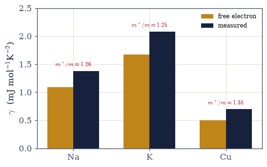
Fig. 658 The Sommerfeld coefficient, predicted and measured. Free-electron \(\gamma = \pi^2N_Ak_B^2/2\varepsilon_F\) (amber) from each metal’s Fermi energy — no parameters — against the calorimetric values (dark; Ashcroft & Mermin lineage). The free gas lands within 40% everywhere and orders the table correctly (\(\gamma \propto 1/\varepsilon_F\)), and the residual ratios \(\gamma_{\text{meas}}/\gamma_{\text{free}} = 1.26, 1.25, 1.38\) (annotated) define the thermal effective mass \(m^*_{\text{th}}/m\): the electron in a metal moves dressed by the lattice (the bands of §7.12 supply the mechanism) and by its fellows (the interacting dressing, Volume VIII). Since \(\gamma \propto g(\varepsilon_F)\) regardless of dispersion, the measured intercept of Fig. 2’s line is a direct reading of the density of states at the Fermi surface — calorimetry as spectroscopy, once more.

Validation 4

✓  the free-electron Sommerfeld coefficients of real metals, from ε_F alone   [max|Δ| = 0.000268988 (rtol=0.01, atol=1e-09)]
✓  the thermal effective masses: m*/m = 1.25–1.38 — the dressing, measured   [ratios [1.26, 1.25, 1.38]]

True

Exercise 5 — The experimenter’s plot

\(C/T\) against \(T^2\): the straight line every low-temperature paper shows, and the 3-kelvin crossover that explains it. Cite Eq. 737.

1. Assemble \(C(T) = \gamma T + AT^3\) for copper with \(A = 12\pi^4R/5\theta_D^3\) (\(\theta_D = 343\) K; the \(T^3\) law invoked, derivation deferred to §7.16) and \(\gamma\) from Exercise 4.

2. Plot \(C/T\) vs \(T^2\) for \(T = 0.5\)–\(5\) K and confirm the straight line with intercept \(\gamma\) and slope \(A\) (waypoints \(0.551, 0.696, 1.274\) mJ mol⁻¹K⁻² at \(1, 2, 4\) K).

3. Compute the crossover \(T^* = \sqrt{\gamma/A} = 3.23\) K and the room-temperature phonon dominance (\(\sim10^2\times\)).

4. State the experimental moral (prose): \(\gamma\) is a liquid-helium quantity — the electron gas speaks only below the phonons’ \(T^3\) roar, which is why Sommerfeld’s coefficient waited for cryogenics.

copper: γ = 0.503 mJ/(mol K²),   A = 0.0482 mJ/(mol K⁴)
  C/T at 1 K: 0.551 mJ/(mol K²)
  C/T at 2 K: 0.696 mJ/(mol K²)
  C/T at 4 K: 1.274 mJ/(mol K²)

T* = √(γ/A) = 3.23 K
at 300 K the lattice (≈3R) outweighs the electrons by 165×

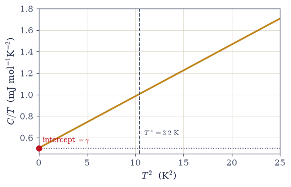
Fig. 659 The experimenter’s plot: \(C/T\) against \(T^2\) for copper at liquid-helium temperatures. The two-power law \(C = \gamma T + AT^3\) (electrons + phonons, the \(T^3\) invoked from experiment and derived in §7.16) becomes a straight line whose intercept is the Sommerfeld coefficient \(\gamma\) (red) and whose slope is the Debye \(A\) — this is how every measured \(\gamma\) in Exercise 4’s table was actually read off. The electron–phonon crossover \(T^* = \sqrt{\gamma/A} = 3.2\) K (marked) divides the plot: below it the electrons dominate the heat capacity, above it the lattice does — by \(\sim10^2\) at room temperature, which is why Drude’s missing heat stayed missing for a generation and why the electron gas speaks only to cryogenic calorimetry.

Validation 5

✓  the electron–phonon crossover: why γ lives below 3 K   [got 3.23132 vs expected 3.23 (rtol=0.02, atol=1e-09)]
✓  the experimenter's line: C/T = γ + AT² at the verified waypoints   [max|Δ| = 0.000380088 (rtol=0.01, atol=1e-09)]

True

Exercise 6 — Pauli paramagnetism, computed honestly

Two shifted bands, one re-solved \(\mu\) — and the second mystery falls. In a field the spin-\(\sigma\) band’s energies shift by \(-\sigma\mu_BB\), which is the same arithmetic as giving that band the chemical potential \(\mu + \sigma B\) and leaving its energies alone; each band then carries half the density of states, \(g/2\). The total number constraint \(N_\uparrow + N_\downarrow = 1\) re-fixes \(\mu\) at every field — skipping that re-solve is the frozen-\(\mu\) error of Exercise 3 wearing a magnet — and \(M\) is the integrated band imbalance. \(M\) is odd in \(B\), so an antisymmetric difference \([M(B) - M(-B)]/2B\) cancels every even error term for free; the window \(B = 10^{-3}\) is the stated compromise, small enough that the \(O(B^2)\) nonlinearity is \(\sim10^{-6}\) relative and large enough that quadrature noise on \(M\) is invisible after the division. Cite Eq. 738.

1. Write magnetization(B, t), the two-band magnetization \(M = (N_\uparrow - N_\downarrow)\mu_B\) per particle: brentq on the total-number constraint, then the difference of the two bands’ split-quad integrals. Write this one yourself — the implementation is the lesson.

2. Write susceptibility(t, B_window=1e-3), extracting \(\chi = \partial M/\partial B\) at \(B = 0\) by the antisymmetric difference above.

3. Verify \(\chi = \mu_B^2g(\varepsilon_F)\) (reduced: \(\tfrac32\)) at \(t = 0.02\).

4. Confirm the Sommerfeld drift \(\chi(t) = \chi_P[1-(\pi^2/12)t^2]\) against the exact computation at \(t = 0.02, 0.05, 0.1\) — five-digit agreement where the expansion holds.

5. Quantify and interpret (prose + number): \(\chi_P/\chi_{\text{Curie}} = \tfrac32 T/T_F = 0.55\%\) at 300 K in copper — metals are feeble, temperature-blind paramagnets because moments beneath the surface face Pauli-occupied partners; the moment of §6.18 finally has its temperature. Landau’s \(-\chi_P/3\) orbital counterpart named, with the honest note that measured metallic \(\chi\) is the Pauli–Landau–core sum.

χ(t = 0.02) by the two-band computation: 1.499506
the Pauli value μ_B² g(ε_F) (reduced):   1.500000

the Sommerfeld drift of χ:
  t = 0.02:  exact = 1.499506   Sommerfeld = 1.499507

  t = 0.05:  exact = 1.496887   Sommerfeld = 1.496916

  t = 0.1:  exact = 1.487125   Sommerfeld = 1.487663

χ_P/χ_Curie at 300 K in copper: (3/2)·T/T_F = 0.55%

Validation 6

✓  Pauli paramagnetism: flat, small, and five digits of Sommerfeld at t = 0.02   [got 1.49951 vs expected 1.49951 (rtol=1e-05, atol=1e-09)]
✓  the (π²/12)t² drift confirmed against the exact two-band computation (t⁴ term allowed for)   [max|Δ| = 0.000537701 (rtol=0.0005, atol=1e-09)]

True

Exercise 7 — One gas, both worlds

\(\mu\), \(C\), and \(\chi\) swept across two decades of temperature — every limiting law already owned by an earlier notebook. Cite Eq. 739.

1. Run the exact machinery you built — your mu_of_T (Exercise 1), heat_capacity (Exercise 2), and susceptibility (Exercise 6) — for \(t = 0.02 \to 6\) and tabulate \(\mu(t)\), \(C(t)\), \(\chi(t)\) (the Setup quad limits and steps apply; the slow region near \(t \sim 1\) noted).

2. Verify the four corners: \(C \to (\pi^2/2)t\) (Sommerfeld) and \(\to \tfrac32\) (classical; \(1.493\) at \(t = 6\)); \(\chi \to \tfrac32\) flat (Pauli) and \(\to 1/t\) (Curie; \(\chi\cdot t = 0.977\) of Curie at \(t = 5\)).

3. Verify \(\mu\)’s landing: against the classical \(\mu = t\ln[(4/3\sqrt\pi)t^{-3/2}]\) of §7.8 at \(t = 3\), with the remaining gap identified as virial-order.

4. Read the triptych (prose): one gas, three observables, eight limits — degeneracy is not a different theory but a regime, and the course now owns the road between.

   t       μ         C         χ
  0.02   +0.9997   0.0986    1.4995
  0.05   +0.9979   0.2449    1.4969
  0.10   +0.9916   0.4772    1.4871
  0.20   +0.9646   0.8397    1.4416
  0.35   +0.8804   1.1248    1.3152
  0.60   +0.6249   1.3088    1.0766
  1.00   -0.0215   1.4055    0.7933
  1.60   -1.3743   1.4520    0.5531
  2.50   -3.9800   1.4751    0.3749
  3.00   -5.6446   1.4810    0.3172
  4.00   -9.3237   1.4876    0.2420
  5.00  -13.3754   1.4911    0.1954
  6.00  -17.7254   1.4932    0.1637

C(6) = 1.4932   (classical 3/2: equipartition recovered in full)
χ(5)·5 = 0.9768   (Curie: 1 — the classical law recovered)
μ(3) = -5.645   classical asymptote -5.798   (gap = virial order, the ∓nλ³ corrections of §7.8)

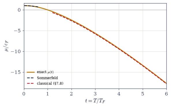
Fig. 660 The level of the sea, from Fermi to Boltzmann. The exact \(\mu(t)\) (amber) with its two limiting laws: Sommerfeld’s parabola \(1-(\pi^2/12)t^2\) (dark dashed), which it hugs to six digits at \(t = 0.02\) and ten parts per million at copper’s room temperature, and the classical \(\mu = t\ln[(4/3\sqrt{\pi})t^{-3/2}]\) of §7.8 (red dashed; the constant derived from the Boltzmann integral, not guessed), which it approaches from above with a virial-order gap. The zero crossing near \(t \approx 1\) marks the dissolution of the sea’s surface: below it a sharp Fermi level organizes the gas, above it the fugacity \(z = e^{\mu/t} < 1\) and Boltzmann bookkeeping takes over. One function, both worlds.

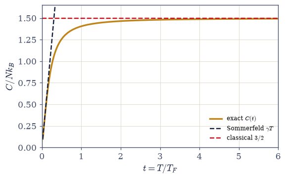
Fig. 661 Drude’s expectation, met on Pauli’s schedule. The exact electronic heat capacity \(C(t)\) (amber) between its two laws: Sommerfeld’s linear \(\gamma T\) (dark dashed) — 1.2% of the classical value at a metal’s operating point — and the classical plateau \(\tfrac32 Nk_B\) (red dashed), reached only when \(T\) climbs past \(T_F\) (\(C = 1.493\) at \(t = 6\)) and every electron is finally free to participate. The knee near \(t \sim 0.5\) is degeneracy lifting: the fraction of electrons Pauli permits to respond grows from \(\sim t\) to all of them. Metals live at \(t \lesssim 0.01\), on the far left edge — which is why the electronic term hides beneath the phonons everywhere except the liquid-helium window of Fig. 2.

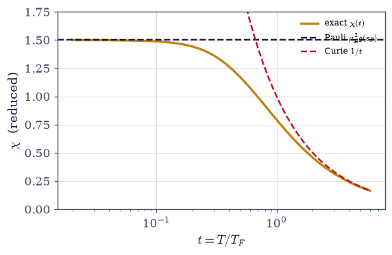
Fig. 662 The second mystery, end to end. The exact spin susceptibility \(\chi(t)\) of the Fermi gas (amber) between its two laws: the Pauli plateau \(\chi = \mu_B^2g(\varepsilon_F)\) (dark dashed) — small, temperature-blind, \(0.55\%\) of Curie’s expectation at a metal’s operating point, because moments beneath the Fermi surface face Pauli-occupied partners — and Curie’s \(1/t\) (red dashed), onto which the exact curve rolls once degeneracy ends and every moment is free (\(\chi\cdot t = 0.98\) of Curie at \(t = 5\)). Classical physics saw only the right half and demanded divergence at low temperature; metals live at \(t \sim 0.004\), deep on the flat left. Landau’s orbital \(-\chi_P/3\) rides on top of this in real metals, with the ion cores’ diamagnetism — the measured value is the sum, stated for honesty.

Validation 7

✓  the full quantum-classical crossover: C reaches the classical 3/2, χ lands on Curie   [max|Δ| = 0.000229218 (rtol=0.01, atol=1e-09)]
✓  μ(3) lands on the classical asymptote of §7.8, to virial order   [got -5.64456 vs expected -5.7978 (rtol=0.03, atol=1e-09)]

True

Exercise 8 — The price list of the Fermi surface

Everything a cold metal does, it does with the thin shell of electrons that Pauli leaves free — and this notebook priced that shell. The chemical potential drifts by parts per million; the heat capacity comes in at one percent of the classical value, linear in \(T\), its coefficient readable off a straight line below three kelvin; the paramagnetism arrives flat and feeble at half a percent of Curie’s demand. Two mysteries that embarrassed the classical theory of metals for a generation turned out to be the same sentence spoken twice. And when the temperature finally climbs past \(T_F\), every suppression lifts on schedule: the gas recovers every classical law and forgets it was ever quantum — the crossover our map (§7.8) promised, now driven end to end.

There is a particular elegance to how the mysteries died. No new force, no new particle — just the realization that in a Fermi sea, almost everyone is forbidden to move. The physics of metals is the physics of the exceptions.

Next, the movement’s summit: the same degeneracy pressure that made copper stiff, asked to hold up a star — and the discovery that above a certain mass, it cannot (§7.11).

Notebook summary

The Fermi sea, warmed by its actual fraction of a percent — and two century-old mysteries dissolved by one sentence: Pauli blocks the bulk; only the surface fraction \(\sim T/T_F\) responds.

• μ(T) Eq. 733: solved exactly by brentq at every temperature; Sommerfeld’s \(1-(\pi^2/12)t^2\) met at six digits (\(t = 0.02\)), departed from honestly at \(t = 0.1\); ten parts per million at copper’s room temperature; and the full arc followed through \(\mu = 0\) onto the classical \(t\ln[(4/3\sqrt\pi)t^{-3/2}]\) of §7.8 — the asymptote’s constant derived, the remaining gap identified as virial-order.

• The estimate Eq. 734: fraction \(T/T_F\), energy \(k_BT\) each — \(C\) verified linear at small \(t\); every exact result below is this picture, dressed.

• The linear heat capacity Eq. 735: the exact derivative (μ re-solved — the frozen-μ trap demonstrated, tens of percent wrong with no warning) meets \((\pi^2/2)t\) at 0.1%; Drude’s mystery quantified — copper’s electrons supply \(1.2\%\) of the classical value at 300 K, scaled by Pauli’s factor \(T/T_F\).

• The γ table Eq. 736: \(1.091, 1.668, 0.503\) vs measured \(1.38, 2.08, 0.695\) mJ mol⁻¹K⁻² — right scale, right ordering, and the ratios defining \(m^*_{\text{th}}/m = 1.25\)–\(1.38\): the dressed electron, previewing the bands of §7.12.

• The experimenter’s plot Eq. 737: \(C/T\) vs \(T^2\), intercept \(\gamma\); the crossover \(T^* = 3.23\) K and the \(\sim10^2\times\) phonon dominance at 300 K — why \(\gamma\) is a liquid-helium quantity (the \(T^3\) invoked; §7.16 derives it).

• Pauli paramagnetism Eq. 738: the honest two-band computation lands on \(\mu_B^2g(\varepsilon_F)\) with the Sommerfeld drift confirmed to five digits; \(0.55\%\) of Curie at room temperature — the feeble, temperature-blind paramagnetism of metals, explained; Landau’s \(-\chi_P/3\) named, the measured sum stated.

• The capstone sweep Eq. 739: \(\mu\), \(C\), \(\chi\) from \(t = 0.02\) to \(6\) — \(C \to 1.493\) (the classical plateau reached), \(\chi\cdot t \to 0.98\) of Curie, all eight limits owned by earlier notebooks. Degeneracy is a regime; the road between is driven.

The physics of metals is the physics of the exceptions.

Outlook

• The summit (§7.11). White dwarfs, the relativistic gas, and the Chandrasekhar mass — the pressure of §7.9 and this notebook’s machinery at stellar scale.

• Where m* comes from (§7.12, §7.13). The sea meets a lattice: bands, and degenerate doping.

• The lattice’s own thermodynamics (§7.16). The Debye \(T^3\), derived — the slope of the experimenter’s plot earns its coefficient.

• Localized moments (§7.18). Curie and Brillouin done properly, where moments are free and the \(1/T\) law is the whole story.

• Horizons, named. Landau levels, Landau diamagnetism, and the de Haas–van Alphen window onto Fermi surfaces; the interacting dressing of \(m^*\) (Volume VIII).

• Cross-reference §7.3 (Sommerfeld, home ground), §7.9 (the sea and its scales), §7.8 (the classical asymptote and the map), §7.7 (\(n_F\)), §6.18 (the moment, put to work), §5.5/§5.6 (the classical laws, recovered on schedule).

Take this notebook with you

Use the download button (↓) in the toolbar above to save this notebook and run it yourself. The published notebooks ship without worked solutions; if you would like the reference solutions — to teach from or to check your own work — get in touch: hello@ramador.me.