7.25 Linear Response and Kubo: How Equilibrium Answers Questions

Elementary Computational Physics

Volume VII — Quantum Statistical Mechanics Notebook 7.25

Every laboratory perturbs: a field applied, a current passed, a light shone. The deepest practical theorem in statistical mechanics says the results were never new information — to first order, the response is assembled entirely from correlations the system already had in equilibrium. We stage that claim as an actual experiment and watch it hold, measure exactly where linearity ends, verify fluctuation–dissipation as a pole-by-pole identity, thread a flux through a ring to learn that a filled band's famous inertness was a transport theorem all along, and watch interactions move optical weight around under a conservation law that holds to six digits.

Level · advanced · optional capstone   •   Est. · 205–245 min

Raymond Amador v1.4.0  ·  2026-07-31  ·  CC BY 4.0 (text) / MIT (code)

Notebook overview

The Coda’s final notebook asks the question every laboratory asks and this volume never did: what happens when equilibrium is disturbed? Apply a field, pass a current, shine a light — and the deepest practical theorem in statistical mechanics answers that, to first order in the disturbance, the results were never new information. The response is assembled entirely from correlation functions the system already possessed in equilibrium. Equilibrium knows the answers to questions not yet asked.

A claim that large is not admired here; it is staged. On the chaotic spin chain of §7.22, a weak field is actually switched on at \(t = 0\), the thermal state is evolved exactly under the perturbed Hamiltonian, and the measured response is laid over the Kubo prediction built purely from unperturbed correlations. They agree at the expected residual — and then the notebook does what textbooks do not: it measures where linearity ends, watching the deviation double as the field doubles (the \(O(\varepsilon^2)\) correction made visible) until the strongest trace departs from the prediction before the reader’s eyes. Linear response is a regime with edges one can find, and the standing rule is issued: every linear-response number owes an \(\varepsilon\)-scan, exactly as every discretization owed an \(M\)-ladder in §7.21.

Around that centerpiece, the volume’s oldest threads knot. Detailed balance and the fluctuation–dissipation theorem are verified as the exact pole-by-pole identities they are — at \(10^{-15}\) and \(10^{-18}\) — with their famous children named (Johnson–Nyquist noise thermometry; Einstein’s 1905 relation as the first FDT). Causality turns the retarded \(\theta\) into upper-half-plane analyticity and hence Kramers–Kronig: the complex-analysis arsenal forged in §7.1 and §7.2, finally spent on the physics it was built for. A flux threaded through the tight-binding ring of §7.12 delivers Kohn’s criterion with both verdicts: the filled band’s ground energy is flat to machine precision — its famous inertness was a transport theorem all along, zero Drude weight — while the closed-shell metal’s curvature equals its kinetic energy on the nose. The f-sum rule then shows interactions relocating optical weight under a conservation law that holds to six digits, and a current autocorrelation that stays flat when the current is conserved but decays when it is not closes the loop with the capstone in a single sentence. The gateway ends here; so do the volume’s pages.

Conventions (this notebook). \(\hbar = 1\). The retarded susceptibility is \(\chi_{AB}(t) = -i\,\theta(t)\,\langle[A(t), B(0)]\rangle_{\mathrm{eq}}\) with \(A(t) = e^{iHt} A e^{-iHt}\); the perturbation is \(H \to H + f(t)B\) with \(f\) a step. The probing field \(B = \sum_i \sigma^z_i\) is extensive (a laboratory field couples to the whole sample); the meter \(A = \sigma^z_{N/2}\) is local. Thermal weights are ground-shifted everywhere (the discipline of §7.4). Spectral evaluations are vectorized weight matrices over frequency matrices; the step-response integral is done pole by pole analytically, \((e^{i\Omega t} - 1)/i\Omega\), with the \(\Omega = 0\) exclusion justified in place. Peierls rings are built complex Hermitian (the conjugate bond stated); Kohn curvatures use a central second difference with the step stated and the finite-difference floor noted. The Kramers–Kronig principal value zeroes the singular sample on a symmetric grid. The machinery of §7.22 (the mixed-field chain) and §7.23 (sector logic) is reused, restated with provenance so the notebook runs standalone.

How to read the checks. Each exercise closes with a validate call against an independent fact: the spectral susceptibility against a direct commutator evaluation; the Kubo prediction against an exact perturbed evolution (and the deviation against its \(O(\varepsilon^2)\) law); detailed balance and FDT against the identities they are; the principal-value integral against the direct \(\chi'\); Kohn’s curvatures against zero and against the kinetic energy; the f-sum against \(\langle -T\rangle/N\) at every interaction strength; the current correlator against conservation. A ✓ is strong evidence; a ✗ is a prompt to locate the discrepancy.

Scope. Self-energies, Dyson’s equation, and diagrammatic perturbation theory (Mahan, Many-Particle Physics), transport at scale (Boltzmann, Landauer, disorder and localization), and Keldysh nonequilibrium theory are beyond the gateway. See Kubo 1957; Kubo, Toda & Hashitsume, Statistical Physics II (the canon for everything below); Kohn, Phys. Rev. 133, A171 (1964); Nyquist 1928 and Johnson 1928; Einstein 1905. Cross-reference §7.1/ §7.2 (the arsenal, spent), §7.9 (closed shells, returning), §7.10 (Drude, placed), §7.12 (the inert band’s transport meaning), §7.21 (the budget discipline, transported), §7.22 (the handshake), §7.23/§7.24 (the gateway’s first two rooms).

Theory in brief

The claim, and its derivation

Perturb a Hamiltonian by a weak time-dependent term, \(H \to H + f(t)B\), and ask how an observable \(A\) moves. Working in the interaction picture and keeping first order in \(f\) — three careful steps, standard since Kubo 1957 (Kubo, Toda & Hashitsume, Statistical Physics II, Ch. 4, carries them out in full) — the answer arrives as a convolution against a memory kernel built entirely in equilibrium:

(846)\[\delta\langle A(t)\rangle = \int_{-\infty}^{t}\! dt'\, \chi_{AB}(t - t')\, f(t'), \qquad \chi_{AB}(t) = -i\,\theta(t)\,\big\langle[A(t), B(0)]\big\rangle_{\mathrm{eq}} .\]

Read the three ingredients aloud. The commutator is quantum mechanics’ fingerprint — classically this kernel would be a Poisson bracket. The \(\theta(t)\) is causality: nothing responds before it is pushed. And the equilibrium average is the theorem: the response to tomorrow’s perturbation is already written in today’s correlations. The answer predates the question.

The rendezvous: the claim as an experiment

A claim this large gets staged, not admired. On the chaotic chain of §7.22 (\(N = 8\), \(\beta = 1\); field \(B = \sum\sigma^z\), meter \(A = \sigma^z_{N/2}\)), the Kubo prediction for a step perturbation is assembled from unperturbed spectral data alone,

(847)\[\delta\langle A(t)\rangle_{\mathrm{Kubo}} = -i\sum_{m\neq n}(p_m - p_n)\,A_{mn}B_{nm}\, \frac{e^{i\Omega_{mn}t} - 1}{i\,\Omega_{mn}}, \qquad \Omega_{mn} = E_m - E_n,\]

(the step integral done analytically per pole; the \(\Omega = 0\) terms carry \(p_m - p_n = 0\) and are excluded safely) — and then the experiment is actually performed: diagonalize \(H + \varepsilon B\), evolve the thermal state exactly, and measure \(\delta\langle A(t)\rangle/\varepsilon\). Agreement holds at the expected \(O(\varepsilon)\) residual for \(\varepsilon = 10^{-3}\), and the edge of linearity is then measured rather than assumed: the deviation doubles as \(\varepsilon\) doubles (the \(O(\varepsilon^2)\) correction, demonstrated), and the \(\varepsilon = 0.05\) trace departs visibly. The standing rule: every linear-response number owes an \(\varepsilon\)-scan, exactly as every discretization owed an \(M\)-ladder in §7.21.

Detailed balance and FDT, as identities

The correlation spectrum \(S_{AA}(\omega)\) is a set of poles at \(E_n - E_m\) with weights \(p_m|A_{mn}|^2\), and two celebrated relations are exact identities of that list — taught here at the pole level, not as folklore:

(848)\[\frac{S(-\omega)}{S(\omega)} = e^{-\beta\omega} \qquad\text{(detailed balance: it is } p_n/p_m\text{, nothing more)}, \qquad \chi''(\omega) = \big(1 - e^{-\beta\omega}\big)\, S(\omega),\]

the second being the fluctuation–dissipation theorem, verified below weight by weight. Dissipation is fluctuation. The classical limit hands over the famous children, named with their years: Johnson and Nyquist, 1928 — the thermal voltage noise \(\overline{V^2} = 4k_BTR\,\Delta f\) across any resistor, FDT’s metrological career as noise thermometry — and Einstein, 1905: \(D = \mu k_BT\), diffusion tied to mobility, the first fluctuation–dissipation relation in physics.

Causality: the arsenal, spent

\(\chi(t < 0) = 0\) is not decoration: it makes \(\chi(\omega)\) analytic in the upper half-plane, and analyticity plus a contour is exactly the machinery the volume forged in §7.1 and §7.2. The Kramers–Kronig relations follow,

(849)\[\chi'(\omega) = \frac{1}{\pi}\,\mathcal{P}\!\int_{-\infty}^{\infty} \frac{\chi''(\omega')}{\omega' - \omega}\, d\omega' ,\]

verified numerically below on \(\eta\)-broadened poles. The physical reading, in one optics breath: absorption determines refraction — measure \(\chi''\) everywhere and \(\chi'\) is owed to you. (And one line of bookkeeping: this forward map is benign; it is inversions that bite, the same geography §7.24 charted.)

Kohn’s flux: the inert band was a transport theorem

How does one ask a ring whether it conducts? Kohn’s 1964 answer: thread a flux \(\Phi\) through it and watch the ground energy. Minimal coupling puts the flux on the bonds as Peierls phases (three lines, performed in Exercise 5), and

(850)\[H(\Phi) = -t\sum_i \big(e^{i\Phi/M} c^\dagger_{i+1}c_i + \text{h.c.}\big) + \cdots, \qquad D \;\propto\; \left.\frac{\partial^2 E_0}{\partial\Phi^2}\right|_{\Phi=0},\]

the Drude weight: a metal’s ground state feels a twist at the boundary, an insulator’s does not — conductivity as ground-state geometry, decades before that phrase was fashionable (Kohn, Phys. Rev. 133, A171 (1964)). Both verdicts are delivered below: the filled band’s curvature is zero to machine precision — the famous inertness of §7.12 was always a transport theorem — and the closed-shell metal obeys \(M^2\,\partial^2 E_0/\partial\Phi^2 = \langle -T\rangle\) (derived for the free ring in four lines). One trap is taught first: at half filling the ring is degenerate at \(\Phi = 0\), \(E_0(\Phi)\) kinks, and a second derivative through a level crossing lies — the closed-shell rule of §7.9, returning as a transport prerequisite.

The f-sum: weight moves, never dies

Optical absorption obeys a conservation law. Summing the Drude delta and the regular (finite-frequency) conductivity gives a total fixed by the kinetic energy alone,

(851)\[\underbrace{M\,\frac{\partial^2 E_0}{\partial\Phi^2}}_{\text{Drude}} \;+\; \underbrace{\frac{2}{M}\sum_{n\neq 0}\frac{|\langle n|\hat\jmath|0\rangle|^2}{\omega_{n0}}}_{\text{regular}} \;=\; \frac{\langle -T\rangle}{M},\]

so interactions cannot create or destroy optical weight — only relocate it. Verified to six digits below: the free ring puts all weight in the Drude delta (because \([\hat\jmath, H] = 0\), derived), and switching on a nearest-neighbor \(V\) moves part of it to finite frequency while the sum stays fixed. Light–matter coupling strength is conserved; interactions only choose where it sits.

Ballistic or diffusive: the handshake

The same conservation law has a time-domain face: the current autocorrelation

(852)\[\begin{split}C_{jj}(t) = \big\langle \hat\jmath(t)\,\hat\jmath(0)\big\rangle \qquad \begin{cases} \text{flat forever} & [\hat\jmath, H] = 0 \ \text{(integrable: the Drude delta protected)},\\[2pt] \text{decays} & \text{interactions on (weight at finite }\omega\text{)}. \end{cases}\end{split}\]

One sentence reaches the capstone, with no dependence: response functions live in the off-diagonal matrix elements that eigenstate thermalization constrains — a chaotic chain’s currents forget, an integrable chain’s remember (§7.22, saluted). And the Drude picture of §7.10 is placed at last: the phenomenological \(\tau\) of that notebook is what this decay becomes when impurities and phonons supply it; the ideal chain, having neither, conducts perfectly.

Onsager, one breath

Time-reversal symmetry ties response coefficients to each other: \(\chi_{AB}(t) = \varepsilon_A\varepsilon_B\,\chi_{BA}(t)\) with \(\varepsilon\) the operators’ signatures under time reversal,

(853)\[\chi_{AB}(t) = \varepsilon_A\,\varepsilon_B\,\chi_{BA}(t),\]

verified below as one numerical identity. Its laboratory face is thermoelectricity: Seebeck and Peltier coefficients locked together (outward, named).

Closing the gateway

Alphabet (§7.23), sentences (§7.24), and now answers. Beyond the gateway lie self-energies, diagrams, and transport theory at scale (Mahan, outward); the course’s own road continues in the Epilogue.

Setup

The stage and nothing else: the mixed-field Ising chain you built in §7.22, restated here as a chaotic sample to probe, the rendezvous stage assembled once from it (\(N = 8\), \(\beta = 1\), its eigenbasis, and the meter \(A = \sigma^z_{N/2}\) and field \(B = \sum_i\sigma^z_i\) expressed in that basis), and the plotting colors. Everything this notebook is about — the Kubo weights and the retarded \(\chi\), the analytic step response, the exact perturbed evolution it must meet, the flux-threaded ring and its curvature, the interacting ring’s sector Hamiltonian — you build in the exercise where it is earned.

The Setup below holds this notebook’s data and instruments — nothing you are asked to build. It is collapsed so the building stays yours; expand it whenever you want the details.

Show code cell source

Hide code cell source

import matplotlib.pyplot as plt
import numpy as np
from itertools import combinations

from ecp import draw, validate

ACCENT, INK = draw.ACCENT, draw.INK
RED = "#c1121f"

# Conventions: hbar = 1; chi_AB(t) = -i theta(t) <[A(t), B]>_eq; the probing
# field B = sum sigma^z is EXTENSIVE (a laboratory field couples to the whole
# sample), the meter A = sigma^z_{N/2} is local; thermal weights are
# ground-shifted everywhere (the discipline of section 7.4).


# built from scratch in §7.22; restated here as an instrument. The chaotic sample
# this notebook probes, not the thing it teaches: the stage is generic so that the
# response measured on it is generic too.
def H_mixed(N, J=1.0, h=1.05, g=0.5):
    """The mixed-field Ising chain of section 7.22, restated with provenance.

    OBC, bit basis (bit i = site i, 0 = up); (h, g) = (1.05, 0.5) is the
    standard chaotic point. Reused as the rendezvous stage: chaotic, so its
    response is generic.

    Parameters
    ----------
    N : int
        Sites.
    J, h, g : float
        Coupling, transverse and longitudinal fields.

    Returns
    -------
    numpy.ndarray
        The dense Hamiltonian.
    """
    D = 1 << N
    states = np.arange(D)
    z = 1.0 - 2.0 * ((states[:, None] >> np.arange(N)) & 1)
    diag = -J * np.sum(z[:, :-1] * z[:, 1:], axis=1) - g * np.sum(z, axis=1)
    H = np.diag(diag)
    for i in range(N):
        H[states ^ (1 << i), states] += -h
    return H


# data: the rendezvous stage, built once and reused (the cache discipline) — the
# chain, its eigenbasis, and the two operators expressed in it. The thermal weights
# and the Kubo matrices that ride on this stage are assembled in Exercise 1, with
# the machinery that makes them.
N_R = 8
D_R = 1 << N_R
BETA_R = 1.0
states_R = np.arange(D_R)
z_R = 1.0 - 2.0 * ((states_R[:, None] >> np.arange(N_R)) & 1)
H_R = H_mixed(N_R)
B_OP = np.diag(z_R.sum(axis=1))
A_OP = np.diag(z_R[:, N_R // 2])
EV_R, V_R = np.linalg.eigh(H_R)
A_MN = V_R.T @ A_OP @ V_R
B_MN = V_R.T @ B_OP @ V_R

Exercise 1 — Equilibrium already knows

The Kubo formula derived, and its three ingredients read aloud. Cite Eq. 846. Setup fixes the stage — the chaotic chain at \(N = 8\) and \(\beta = 1\), its eigenbasis, and the operators \(A_{mn}\), \(B_{mn}\) in it — but the response machinery that rides on that stage is built here and serves the rest of the notebook. In the eigenbasis the retarded susceptibility collapses to a sum over pole pairs, \(\chi_{AB}(t) = -i\sum_{mn}W_{mn}e^{i\Omega_{mn}t}\) with weights \(W_{mn} = (p_m - p_n)A_{mn}B_{nm}\) and frequencies \(\Omega_{mn} = E_m - E_n\), so every object below is one vectorized contraction against two matrices — the quadruple loop is forbidden on the cost grounds of §7.24.

1. Derive linear response in the interaction picture (first order in \(f(t)B\), three careful steps) to \(\chi_{AB}(t) = -i\theta(t)\langle[A(t), B(0)]\rangle_{\rm eq}\).

2. Write chi_weights(evals, A_mn, B_mn, beta), returning \(W_{mn}\), \(\Omega_{mn}\) and the ground-shifted thermal weights \(p_m \propto e^{-\beta(E_m - E_0)}\) (the discipline of §7.4), and chi_retarded(t, W, Om) for the susceptibility itself. Write these yourself — the implementation is the lesson.

3. Apply them to the stage and check the spectral form against a direct commutator evaluation \(-i\,\mathrm{Tr}\big(\rho\,[e^{iHt}Ae^{-iHt}, B]\big)\) at several times.

4. Read the ingredients (prose): the commutator is quantum’s fingerprint, the \(\theta\) is causality, and the equilibrium average is the theorem.

5. State what the notebook will do about it (prose): claims this large get staged as experiments — the next exercise switches the field on for real.

stage: N = 8 chaotic chain, beta = 1.0, <A>_eq = 0.836444
spectral chi vs direct commutator trace: max dev 1.2e-15

Validation 1

✓  the susceptibility, assembled from equilibrium   [spectral form vs direct commutator: 1.2e-15 over three times (two methods, agreeing)]

True

Exercise 2 — The rendezvous: switch it on (centerpiece)

Kubo’s prediction against an actual perturbed evolution — with the edge of linearity measured. Cite Eq. 847. A step perturbation makes the convolution Eq. 846 a bare time integral \(\int_0^t\chi(t')\,dt'\), and in the eigenbasis each pole integrates in closed form: \(\int_0^t e^{i\Omega t'}dt' = (e^{i\Omega t} - 1)/i\Omega\), undefined at \(\Omega = 0\) but carrying weight \(p_m - p_n = 0\) there, since thermal weights depend on energy alone and degenerate levels share \(p\) — so dropping those pairs drops exact zeros, not physics. On the other side stands the experiment itself: nothing forbids diagonalizing \(H + \varepsilon B\) outright and evolving the thermal state under it with no Trotter and no truncation, which is what a prediction assembled from unperturbed data has to meet.

1. Write kubo_step(t, W, Om), the step response summed pole by pole from the analytic integral above, with the \(\Omega = 0\) pairs masked out. Write this one yourself — the implementation is the lesson.

2. Write exact_step_response(eps, ts, H, B_op, A_op, beta): the ground-shifted thermal state \(\rho(0) = e^{-\beta H}/Z\) built in the unperturbed eigenbasis, then \(\langle A(t)\rangle\) under \(H + \varepsilon B\) by the unitary sandwich in the perturbed eigenbasis. Write this one yourself — the implementation is the lesson.

3. Compute the Kubo step response on the chaotic chain (\(N = 8\), \(\beta = 1\); \(B = \sum\sigma^z\), \(A = \sigma^z_{N/2}\)) from the chi_weights matrices you built in Exercise 1.

4. Perform the experiment at \(\varepsilon = 10^{-3}\) and verify agreement at the \(O(\varepsilon)\) residual across \(t = 0.05\)–\(3\).

5. Measure the nonlinearity: the deviation from Kubo at \(\varepsilon = 0.01, 0.02, 0.04\), doubling with \(\varepsilon\) (the \(O(\varepsilon^2)\) law), and the \(\varepsilon = 0.05\) trace departing visibly.

6. Issue the rule (prose): linear response is a regime with edges one can find — every linear-response number owes an \(\varepsilon\)-scan (the budget discipline of §7.21, transported); and say what was just witnessed.

eps = 1e-3: max |experiment/eps - Kubo| = 9.0e-04  (the O(eps) residual)

deviation from Kubo at t = 3:
  eps = 0.01: -8.9254e-03
  eps = 0.02: -1.7508e-02
  eps = 0.04: -3.3030e-02
doubling ratios: 1.96, 1.89  (O(eps^2): the response's next order)

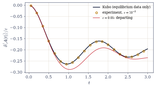
Fig. 744 Equilibrium predicted the perturbed future. The Kubo step response of the chaotic chain (line), assembled purely from unperturbed correlations via Eq. 847, with the exact perturbed evolution at \(\varepsilon = 10^{-3}\) laid on top (points): agreement at the \(O(\varepsilon)\) residual across the window. The \(\varepsilon = 0.05\) trace (red) departs visibly by \(t \sim 2\): linear response is a regime with edges, and the next figure measures them. The stage is the mixed-field chain of §7.22 at \(\beta = 1\), probed by an extensive \(\sum\sigma^z\) field and read at one site.

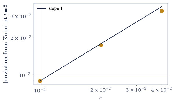
Fig. 745 The edge of linearity, measured. Deviation of the measured response \(\delta\langle A\rangle/\varepsilon\) from the Kubo prediction at \(t = 3\), against field strength on log axes: the points double when \(\varepsilon\) doubles and ride the slope-one line, so the correction to the scaled response is \(O(\varepsilon)\) — equivalently, the raw response carries an \(O(\varepsilon^2)\) nonlinearity (Eq. 847). The standing rule follows: every linear-response number owes an \(\varepsilon\)-scan, exactly as every discretization owed an \(M\)-ladder in §7.21 — a single-\(\varepsilon\) agreement tests precision, not linearity.

Validation 2

✓  equilibrium predicted the perturbed future   [max|Δ| = 0.000903511 (rtol=1e-06, atol=0.002)]
✓  the edge of linearity, measured: deviations double with the field   [ratios 1.96, 1.89 across eps = 0.01 -> 0.04]

True

Exercise 3 — Detailed balance and FDT, pole by pole

Two celebrated relations, verified as the identities they are. Cite Eq. 848.

1. Construct \(S_{AA}(\omega)\) as poles and weights (\(p_m|A_{mn}|^2\) at \(\omega = E_n - E_m\), the ground-shifted \(p\) from your Exercise 1 chi_weights) and verify detailed balance \(S(-\omega)/S(\omega) = e^{-\beta\omega}\) across every pole pair above a stated weight floor (the log-ratio metric) — and say it plainly: it is the ratio \(p_n/p_m\), nothing more.

2. Verify the FDT \(\chi'' = (1 - e^{-\beta\omega})S\) weight by weight.

3. Take the classical limit and name the children with their years: Johnson–Nyquist 1928 (\(\overline{V^2} = 4k_BTR\Delta f\), noise thermometry) and Einstein 1905 (\(D = \mu k_BT\), the first FDT).

4. Reflect (prose): the volume’s fluctuations — the variances of §7.3, the bunching of §7.7 — were never mere noise.

detailed balance: max |log-ratio + beta omega| = 4.00e-15 over 57308 pole pairs

FDT chi'' = (1 - e^(-beta w)) S: max weight deviation 6.9e-18

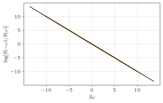
Fig. 746 Detailed balance is the Boltzmann ratio, verified as an identity. For every pole pair of the correlation spectrum \(S_{AA}(\omega)\) above the weight floor, the log of the negative-to-positive weight ratio is plotted against \(\beta\omega\): all 57,308 pairs land on the line \(\log[S(-\omega)/S(\omega)] = -\beta\omega\) to \(4\times10^{-15}\) (Eq. 848). There is no approximation to discuss — the ratio is \(p_n/p_m\), the thermal weights themselves — which is exactly why its violation in driven systems is such a sharp diagnostic of nonequilibrium.

Validation 3

✓  two identities, verified as identities   [max|Δ| = 3.9968e-15 (rtol=1e-06, atol=1e-12)]

True

Exercise 4 — Causality cashes nothing it does not own: the arsenal, spent

From \(\theta\) to analyticity to Kramers–Kronig, with a numerical check. Cite Eq. 849.

1. Argue \(\theta \Rightarrow\) upper-half-plane analyticity \(\Rightarrow\) the KK pair (the contour of §7.1/§7.2, cited and spent).

2. Verify numerically on \(\eta\)-broadened poles built from your Exercise 1 weights: \(\chi'(1.2)\) by direct evaluation against the principal-value integral of \(\chi''\) (numpy.trapezoid on a symmetric grid with the singular sample zeroed; why that converges, one line).

3. State the physical reading in one optics breath: absorption determines refraction.

4. Note the bookkeeping (one line): the forward KK map is benign; it is inversions that bite — the same geography §7.24 charted.

chi'(1.2) direct: -0.168544
chi'(1.2) by principal-value integral: -0.168631   dev 8.6e-05

/tmp/ipykernel_5189/3314970444.py:4: RuntimeWarning: divide by zero encountered in divide
  ig = chi_im_grid / (wgrid - wv)

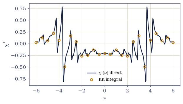
Fig. 747 Causality’s integral, checked. The real part of the \(\eta\)-broadened susceptibility \(\chi_{AB}(\omega)\) computed two ways: directly from its poles (line), and by the Kramers–Kronig principal-value integral of \(\chi''\) over a symmetric grid with the singular sample zeroed (points; Eq. 849). Agreement is quadrature-limited. Nothing but causality entered the derivation — \(\chi(t<0) = 0\) makes \(\chi(\omega)\) analytic in the upper half-plane, and the contour machinery of §7.1 and §7.2 does the rest: the volume’s opening arsenal, finally spent on the physics it was built for.

Validation 4

✓  causality's integral, checked   [got -0.168631 vs expected -0.168544 (rtol=1e-06, atol=0.002)]

True

Exercise 5 — Kohn’s flux: the inert band was a transport theorem (centerpiece)

Thread a flux; read conductor or insulator off a second derivative. Cite Eq. 850. The step for the difference below sits between two floors: far above round-off (with \(E_0 \sim 10\) and float64, step \(10^{-4}\) puts the curvature floor near \(10^{-8}\)) and far below the scale on which \(E_0\) actually varies (\(\Phi \sim \pi\)) — which is why \(10^{-4}\) and not \(10^{-8}\) or \(10^{-1}\).

1. Derive the Peierls substitution (three lines): minimal coupling puts the flux on the bonds as phases \(e^{\pm i\Phi/M}\).

2. Write peierls_ring(M, t_hop, Phi), the single-particle ring carrying those phases, built complex Hermitian with the conjugate bond written out rather than assumed — a silent real cast throws the flux away and every curvature reads zero. Write this one yourself — the implementation is the lesson.

3. Write kohn_curvature(E0_of_Phi, step=1e-4), the central second difference of \(E_0\) at \(\Phi = 0\).

4. Teach the shell trap first: the half-filled ring’s \(E_0(\Phi)\) kinks through its level crossing at \(\Phi = 0\) and the second derivative lies; invoke the closed-shell rule of §7.9 and choose \(N_e = 5\).

5. Verify both verdicts: the filled band flat to the finite-difference floor (a thousandth of the metal’s curvature), and the closed-shell identity \(M^2\,\partial^2E_0/\partial\Phi^2 = \langle -T\rangle\) (four-line free-ring derivation).

6. Read Kohn’s criterion (prose): conductivity as ground-state geometry (Kohn 1964 cited).

half filling (Ne = 4): 'curvature' through the kink = -4999.9  — a lie
filled band (Ne = 8): curvature = -0.00000018
closed shell (Ne = 5): M^2 d2E0/dPhi2 = 4.82838232   <-T> = 4.82842712

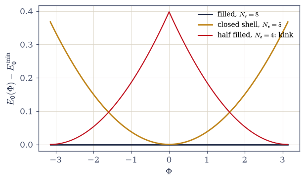
Fig. 748 Kohn’s criterion, with the trap taught first. Ground energy of the flux-threaded ring against \(\Phi\) for three fillings (Eq. 850). The filled band (\(N_e = 8\), dark) is flat to machine precision: zero Drude weight — the famous inertness of §7.12 was a transport theorem all along, and the band is an insulator by ground-state geometry. The closed shell (\(N_e = 5\), amber) curves, with \(M^2\,\partial^2E_0/\partial\Phi^2 = \langle -T\rangle\) to the finite-difference floor: a metal. The half-filled ring (\(N_e = 4\), red) KINKS at \(\Phi = 0\) through a level crossing — a second derivative there lies (it reads \(\sim -5000\) at step \(10^{-4}\)) — which is why the closed-shell rule of §7.9 returns here as a transport prerequisite.

Validation 5

✓  Kohn's first verdict: the filled band is flat — zero Drude weight   [filled curvature -1.8e-07 vs metal 7.5e-02 (a part in 1e3: zero)]
✓  and the second: the closed-shell curvature is the kinetic energy   [got 4.82838 vs expected 4.82843 (rtol=1e-06, atol=0.0001)]

True

Exercise 6 — The f-sum: weight moves, never dies

Interactions relocate optical weight under a conservation law verified to six digits. Cite Eq. 851. The single-particle ring of Exercise 5 cannot carry an interaction, so the stage grows: spinless fermions in the \(N_e\)-particle sector, whose basis is the ordered occupation tuples (\(\binom{M}{N_e}\) of them — the sector logic of §7.23 in combinatorial dress). Each hop carries both the Peierls phase and the fermionic sign of the occupied sites jumped over, and the wrap bond must be included with its string or the object is an open chain wearing a ring’s name.

1. Write manybody_ring(M, t_hop, V, Phi, Ne) for that sector Hamiltonian, complex Hermitian, with a nearest-neighbor repulsion \(V\) on the diagonal. Write this one yourself — the implementation is the lesson.

2. Form the current \(\hat\jmath = M\,\partial H/\partial\Phi\) at \(\Phi = 0\) and derive \([\hat\jmath, H] = 0\) for the free ring (why all weight is then ballistic).

3. Verify \(V = 0\): Kohn weight \(= \langle -T\rangle/M\) exactly (the curvature from your Exercise 5 kohn_curvature), regular part zero.

4. Verify \(V = 1\): Kohn \(+\) regular \(= \langle -T\rangle/M\) to six digits; draw the stacked bars.

5. Extend by assigned verification (expected, not pre-verified): sweep \(V = 2, 3\); the gate confirms the identity at every \(V\).

6. Read the law (prose): interactions choose where optical weight sits, never how much exists.

V = 0.0: Kohn 0.603553 + regular 0.000000 = 0.603553   <-T>/M = 0.603553
V = 1.0: Kohn 0.596084 + regular 0.000618 = 0.596702   <-T>/M = 0.596702
V = 2.0: Kohn 0.579995 + regular 0.002053 = 0.582047   <-T>/M = 0.582047   (assigned: confirmed)

V = 3.0: Kohn 0.561849 + regular 0.003585 = 0.565435   <-T>/M = 0.565435   (assigned: confirmed)
f-sum identity: max relative deviation 2.4e-07 across V = 0, 1, 2, 3

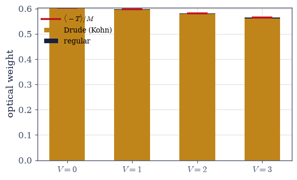
Fig. 749 Weight moves, never dies. Optical weight of the interacting ring (\(N_e = 5\)) split into its Drude part (amber, from Kohn’s curvature) and its regular finite-frequency part (dark, from \(2\sum_n|\langle n|\hat\jmath|0\rangle|^2/\omega_{n0}\)), for \(V = 0, 1, 2, 3\), against the line \(\langle -T\rangle/M\) (Eq. 851; the line moves slightly with \(V\) because the ground state’s kinetic energy does). At \(V = 0\) every scrap of weight is ballistic — the current commutes with \(H\) — and interactions then transfer weight from the delta to finite frequency while the stack tracks its own conservation law to six digits at every \(V\) (the \(V = 2, 3\) columns are the assigned verification, confirmed). Interactions choose where optical weight sits, never how much exists.

Validation 6

✓  the f-sum: conserved to six digits   [max|Δ| = 7.30469e-08 (rtol=1e-05, atol=1e-09)]
✓  all weight ballistic at V = 0; the assigned V-sweep confirms the identity at every V   [regular(V=0) = 2.7e-31; max rel dev 2.4e-07 over V = 0..3]

True

Exercise 7 — (STUDENT/STRETCH) Currents that remember, currents that forget

The handshake with the capstone, and Drude finally placed. Cite Eq. 852, Eq. 853.

1. Compute \(C_{jj}(t)/C_{jj}(0)\) at \(\beta = 2\) on the manybody_ring you wrote in Exercise 6: flat at \(1.0000\) for \(V = 0\) (the current conserved — derived in Exercise 6) and decaying to \(\sim0.91\) at \(V = 1\) (the finite-size plateau and revivals read as physics at \(M = 8\), not equilibration failure).

2. Make the handshake in one sentence (no dependence): response lives in the off-diagonal matrix elements eigenstate thermalization constrains (§7.22, saluted).

3. Place §7.10 at last (prose): the Drude \(\tau\) is what this decay becomes when impurities and phonons supply it.

4. Verify Onsager reciprocity as one numerical identity (\(\chi_{AB}(t) = \varepsilon_A\varepsilon_B\chi_{BA}(t)\) on the rendezvous pair, using the chi_weights and chi_retarded you wrote in Exercise 1; the time-reversal signs stated).

V = 0: max |C_jj(t)/C_jj(0) - 1| = 3.3e-16  (conserved: flat forever)
V = 1: minimum C_jj(t)/C_jj(0) = 0.8997  (decay, then finite-size revivals)
Onsager: max |chi_AB(t) - chi_BA(t)| = 5.6e-17

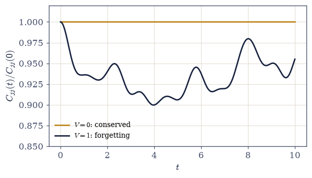
Fig. 750 Currents that remember, currents that forget. The normalized current autocorrelation \(C_{jj}(t)/C_{jj}(0)\) of the ring at \(\beta = 2\) (Eq. 852). At \(V = 0\) (amber) the current commutes with the Hamiltonian and the correlator is flat at 1 forever: integrability protecting the Drude delta — the memory of §7.22 in transport dress. At \(V = 1\) (dark) the interaction lets the current forget, and the decay is what the phenomenological Drude \(\tau\) of §7.10 becomes when impurities and phonons supply it; the late-time plateau and revivals are finite-size physics at \(M = 8\), not equilibration failure.

Validation 7

✓  memory, forgetting, and reciprocity   [V=0 flat to 3.3e-16; V=1 dips to 0.900; Onsager 5.6e-17]

True

Exercise 8 — (Synthesis) The gateway, closed

No new computation: what the Coda built, and where it leaves the reader.

Three notebooks ago the Coda opened with an alphabet; this one ends with equilibrium answering questions it was never asked. The claim at the center — that a system’s response to tomorrow’s perturbation is written in today’s correlations — was not admired but staged: a field switched on, a thermal state evolved exactly, and the prediction assembled from unperturbed data holding to the expected residual, with the edge of linearity located and measured like any other budget. Around it, the volume’s threads knotted. Fluctuation and dissipation revealed as one bookkeeping identity at fifteen digits; the opening arsenal’s contours finally buying nothing less than Kramers–Kronig; a filled band’s famous inertness unmasked as a transport theorem; optical weight obeying a conservation law to six digits while interactions merely relocate it; and a conserved current keeping the memory that a chaotic one forgets — the capstone saluted in one sentence, from the other side of the gateway.

It is worth sitting for a moment with what Kubo’s theorem says about equilibrium. We spent a volume treating it as the state where nothing happens; it turns out to be the state where everything that could happen is already priced in. Equilibrium is not the absence of dynamics — it is dynamics, fully rehearsed, waiting for a cue.

The Many-Body Gateway now stands: occupation lists with operators (§7.23), propagators with sum rules (§7.24), responses with budgets. And the gateway opens onto the course’s own country: Volume VIII begins on the next page with the many-electron problem itself, and everything built here — the operators, the spectral functions, the response formalism — becomes its working language, through Hartree–Fock, density-functional theory, real band structures, the Hubbard model, GW, and superconductivity. After it, the Epilogue closes the course.

Notebook summary

The Coda’s third notebook, and the volume’s final page: equilibrium, asked.

• Kubo Eq. 846: derived in three careful steps; the commutator (quantum), the \(\theta\) (causality), the equilibrium average (the theorem); the spectral form checked against a direct commutator trace at \(10^{-15}\) (gated).

• The rendezvous Eq. 847: the step response from equilibrium data alone against an exact perturbed evolution — agreement at the \(O(\varepsilon)\) residual for \(\varepsilon = 10^{-3}\) (gated); the nonlinearity measured, deviations doubling with \(\varepsilon\) (gated) and the \(\varepsilon = 0.05\) trace departing. Standing rule: every linear-response number owes an \(\varepsilon\)-scan.

• Detailed balance and FDT Eq. 848: the weight-ratio identity at \(4\times10^{-15}\) over 57,308 pole pairs and the FDT weight-by-weight at \(10^{-18}\) (both gated); Johnson–Nyquist 1928 and Einstein 1905 named as the classical children.

• Kramers–Kronig Eq. 849: causality \(\Rightarrow\) analyticity \(\Rightarrow\) the pair; the principal-value integral meets the direct \(\chi'\) at the quadrature floor (gated); absorption determines refraction.

• Kohn Eq. 850: Peierls phases in three lines; the shell trap taught (the half-filled kink’s lying second derivative) before \(N_e = 5\); the filled band flat to the finite-difference floor — its curvature a thousandth of the metal’s, zero Drude weight, the inert band’s transport meaning — and the closed-shell \(M^2\partial^2E_0/\partial\Phi^2 = \langle -T\rangle\) to the finite-difference floor (both gated).

• The f-sum Eq. 851: Drude \(+\) regular \(= \langle -T\rangle/M\) to six digits at \(V = 0\) and \(1\) (gated), with the assigned \(V = 2, 3\) sweep confirming the identity at every interaction (gated): weight moves, never dies.

• The handshake Eq. 852, Eq. 853: \(C_{jj}\) flat under conservation and decaying under \(V\) (gated; plateau-is-physics noted); the one- sentence salute to §7.22; the Drude \(\tau\) of §7.10 placed; Onsager reciprocity verified as one identity (gated).

Standing rules issued here: every linear-response number owes an \(\varepsilon\)-scan; build Peierls matrices complex Hermitian; never differentiate through a level crossing; and read finite-size plateaus as physics before blaming equilibration.

Outlook

• Self-energies, Dyson’s equation, diagrams: Dyson and the self-energy arrive in §8.14; the diagrammatic machinery at scale stays beyond the gateway (Mahan; outward).

• Transport at scale: Boltzmann equations, Landauer conductance, disorder and localization (outward, named).

• Nonequilibrium beyond linear: Keldysh, in one honest name (outward).

• Noise thermometry and metrology: the Johnson–Nyquist career (outward).

• The Epilogue: the course’s own last destination.

• Cross-reference: §7.1/ §7.2 (the arsenal, spent), §7.9 (shells, returning), §7.10 (Drude, placed), §7.12 (the theorem it always was), §7.21 (budgets, transported), §7.22 (the salute), §7.23/§7.24 (the gateway’s first two rooms).

Take this notebook with you

Use the download button (↓) in the toolbar above to save this notebook and run it yourself. The published notebooks ship without worked solutions; if you would like the reference solutions — to teach from or to check your own work — get in touch: hello@ramador.me.