3.3 Gauss’s Law and the Differential Form

Elementary Computational Physics

Volume III — Classical Electrodynamics Notebook 3.3

Flux, symmetry, and the first field equation: Gauss's law in integral and differential form, the fields of the canonical charge geometries, and ∇·E = ρ/ε₀ — the local statement that makes electrodynamics the first classical field theory.

Level · intermediate   •   Est. · 100–130 min

Raymond Amador v1.4.0  ·  2026-07-31  ·  CC BY 4.0 (text) / MIT (code)

Notebook overview

Coulomb’s law (§3.1) gives the field of any charge as a sum, and for a complicated distribution that sum is a chore. Gauss’s law is the shortcut that symmetry earns: it relates the flux of the field through a closed surface to the charge inside, and, whenever the geometry is symmetric enough, hands us the field with almost no work. This notebook develops both faces of the law. The integral form is the global bookkeeping statement, true for any surface; the differential form, \(\nabla\cdot\mathbf E = \rho/\varepsilon_0\), ties the field to its source at a single point and is the first field equation of the volume.

We tour the three symmetry classes the law makes tractable, the spherical, cylindrical, and planar, deriving and computing the field of each canonical geometry: the solid sphere, the shell, the line, the sheet, the capacitor, and the slab. Then we give the numerical divergence sketched at the end of §3.1 its full treatment, confirming \(\nabla\cdot\mathbf E = \rho/\varepsilon_0\) pointwise on a grid. Two threads run alongside the physics. The first is that this volume is, in Landau and Lifshitz’s phrase, the classical theory of fields, and \(\nabla\cdot\mathbf E=\rho/\varepsilon_0\) is the first of the local laws it assembles. The second is the gravitational parallel: the very same law governs any inverse-square field, so a mass dropped down a tunnel through the Earth oscillates, and we compute its period.

Everything is in SI units, with \(\varepsilon_0 = 8.854\times10^{-12}\,\)F/m, \(k = 1/4\pi\varepsilon_0 \approx 8.99\times10^9\,\)N·m²/C², and \(G = 6.674\times10^{-11}\,\)N·m²/kg² for the gravitational thread. Electrostatic fields do not move, so every figure here is a faithful static plot: field lines at equal angular spacing, or arrows whose length and colour encode \(|\mathbf E|\).

How to read the checks. Each exercise ends with a validate call against an independent fact: a flux equal to \(Q_{\text{enc}}/\varepsilon_0\), an interior field that vanishes, a divergence that equals \(\rho/\varepsilon_0\). A ✓ is strong evidence; a ✗ is a prompt to locate the discrepancy, not a verdict.

Scope. A working review, not a full electrodynamics course. The standard references are Nolting, Theoretical Physics 3 [Nol16], and Griffiths, Introduction to Electrodynamics [Gri17] (ch. 2); for the field-theory framing see Landau & Lifshitz, The Classical Theory of Fields [LL80].

Theory in brief

Electric flux

The flux of the field through a surface measures how much of it pierces the surface,

(200)\[\Phi = \oint_S \mathbf E\cdot d\mathbf A ,\]

with \(d\mathbf A\) the outward area element. For a closed surface \(\Phi\) counts the net number of field lines leaving the volume.

Gauss’s law, integral form

The flux through any closed surface depends only on the charge it encloses,

(201)\[\oint_S \mathbf E\cdot d\mathbf A = \frac{Q_{\text{enc}}}{\varepsilon_0} ,\]

independent of the surface’s shape and of every charge outside it. This follows from Coulomb’s \(1/r^2\) and the geometry of solid angle: a point charge sends a fixed flux \(q/\varepsilon_0\) through the full \(4\pi\) of solid angle, and the \(1/r^2\) falloff exactly cancels the \(r^2\) growth of area, so the same flux crosses every surrounding surface (we measured precisely this for a point charge in §3.1).

Using symmetry

When symmetry fixes the field’s direction and makes its magnitude constant over a well-chosen Gaussian surface, the dot product and the integral in Eq. 201 collapse, and the law alone yields \(E\),

(202)\[E \oint_S dA = \frac{Q_{\text{enc}}}{\varepsilon_0} \quad\Longrightarrow\quad E = \frac{Q_{\text{enc}}}{\varepsilon_0\,A} .\]

Three symmetry classes make this work: spherical (a sphere as Gaussian surface), cylindrical (a coaxial cylinder), and planar (a pillbox straddling the charge). We develop all three below.

Gauss’s law, differential form

Shrinking the surface to a point and applying the divergence theorem, \(\oint_S\mathbf E\cdot d\mathbf A=\int_V \nabla\cdot\mathbf E\,dV\), turns the integral law into a local one,

(203)\[\nabla\cdot\mathbf E = \frac{\rho}{\varepsilon_0} .\]

This is the first field equation of the course: a statement, at every point in space, that the divergence of the field is set by the charge density right there. Where charge sits, field lines are born; where space is empty, the field is divergence-free. It is the template for everything that follows.

The field-theory viewpoint

It is worth naming what we are doing. Landau and Lifshitz call this entire subject the classical theory of fields, and electrodynamics is its forerunning and richest example: a physics not of particles and forces-at-a-distance but of a field that fills space and obeys local equations. Equation Eq. 203 is the first of those local laws. The volume assembles the rest one at a time until they close into Maxwell’s equations (§3.8), and the relativistic capstone (§3.12) shows that the electric and magnetic fields are a single object seen from different frames. Reading \(\nabla\cdot\mathbf E=\rho/\varepsilon_0\) as “the first field equation,” rather than “a tidy way to find \(E\),” is the shift of viewpoint this volume is built around.

The gravitational parallel

Gauss’s law needs only the inverse-square form, so gravity obeys it too. With the gravitational field \(\mathbf g\) playing the role of \(\mathbf E\) and mass density \(\rho_m\) the role of charge,

(204)\[\nabla\cdot\mathbf g = -4\pi G\,\rho_m ,\]

the same structure, with \(-4\pi G\) in place of \(1/\varepsilon_0\). The sign is the honest difference: gravity only attracts, so \(\mathbf g\) points toward mass. The field equation is identical, but the phenomenology is not. There is no negative mass, so there is no gravitational “shielding” and no gravitational conductor; the tricks that work for charges on a conductor have no gravitational twin. What does transfer exactly is everything that followed from spherical symmetry, the shell theorem and the \(g\propto r\) interior of a uniform sphere, which we use in Exercise 8 to drop a mass through the Earth.

Setup

Setup holds the SI constants and the two charge colours, the full 3-D point-charge field and the spherical flux integral of §3.1 restated here as tools, and a quiver builder for the field maps. The notebook’s own machinery is not here: you write the cube flux integral in Exercise 1, the closed-form field of each symmetry class as the exercises reach them, and the tunnel equation of motion in Exercise 8.

The Setup below holds this notebook’s data and instruments — nothing you are asked to build. It is collapsed so the building stays yours; expand it whenever you want the details.

Show code cell source

Hide code cell source

import numpy as np
import matplotlib.pyplot as plt
from scipy.integrate import solve_ivp

from ecp import draw, validate

# data: SI constants, shared across Volume III.
from scipy.constants import epsilon_0 as EPS0  # vacuum permittivity, F/m

K = 1.0 / (4.0 * np.pi * EPS0)  # data: Coulomb constant ≈ 8.99e9 N·m²/C²
NANO = 1e-9  # data: 1 nC or 1 nC/m, etc.
from scipy.constants import G as G_GRAV  # data: gravitational constant, N·m²/kg²

POS, NEG = "#c1121f", "#16213e"  # data: positive charge red, negative dark blue


# built from scratch in §3.1 (`E_point`, the same Coulomb field written in the
# z = 0 plane); restated here in full 3-D as an instrument.
def E_point_3d(q, r0, P):
    """Field of a point charge at arbitrary 3-D field points.

    The full 3-D Coulomb field k·q·r̂/r^2, used to integrate flux over a
    surface.

    Parameters
    ----------
    q : float
        Charge in coulombs.
    r0 : array_like
        Source position ``(x, y, z)``.
    P : numpy.ndarray
        Field points of shape ``(..., 3)``.

    Returns
    -------
    numpy.ndarray
        The field vectors at ``P``, same leading shape, in V/m.
    """
    d = P - np.asarray(r0, float)
    r = np.linalg.norm(d, axis=-1)
    with np.errstate(divide="ignore", invalid="ignore"):
        return K * q * d / r[..., None] ** 3


# built from scratch in §3.1 (Exercise 6, where the (θ, φ) trapezoid over a sphere
# was yours to write); restated here as an instrument, generalised to several
# charges at arbitrary positions and to an off-origin sphere.
def flux_through_sphere(charges, Rs, center=(0.0, 0.0, 0.0), n=200):
    """Numerical electric flux through a sphere.

    Integrates the closed-surface integral of E·dA with `numpy.trapezoid` on a
    (θ, φ) grid; by Gauss's law it equals Q_enc/ε0.

    Parameters
    ----------
    charges : list of tuple
        Each ``(q, r0)``: a charge and its 3-D position.
    Rs : float
        Sphere radius.
    center : tuple of float, optional
        Sphere centre (default origin).
    n : int, optional
        Grid resolution per angle (default 200).

    Returns
    -------
    float
        The total flux through the sphere, in V·m.
    """
    c = np.asarray(center, float)
    th = np.linspace(0.0, np.pi, n)
    ph = np.linspace(0.0, 2.0 * np.pi, n)
    TH, PH = np.meshgrid(th, ph, indexing="ij")
    nhat = np.stack(
        [np.sin(TH) * np.cos(PH), np.sin(TH) * np.sin(PH), np.cos(TH)], axis=-1
    )
    P = c + Rs * nhat
    E = np.zeros_like(P)
    for q, r0 in charges:
        E = E + E_point_3d(q, r0, P)
    En = np.sum(E * nhat, axis=-1)  # E · n̂
    integrand = En * Rs**2 * np.sin(TH)  # E·n̂ dA/(dθ dφ)
    return np.trapezoid(np.trapezoid(integrand, ph, axis=1), th)


# instrument: a plotting scaffold — turning a radial magnitude profile into
# quiver arrays is presentation, not the lesson of any exercise here.
def radial_quiver_data(Emag_of_r, xs):
    """Build quiver arrays for a planar radial field of given magnitude.

    Turns a radial magnitude profile E(r) into (X, Y, U, V) with E pointing
    radially, for a faithful field map.

    Parameters
    ----------
    Emag_of_r : callable
        Function ``r -> |E|(r)``.
    xs : numpy.ndarray
        1-D coordinate samples shared by both axes.

    Returns
    -------
    X, Y, U, V : numpy.ndarray
        Meshgrid coordinates and the radial field components on them.
    """
    X, Y = np.meshgrid(xs, xs)
    r = np.hypot(X, Y)
    with np.errstate(divide="ignore", invalid="ignore"):
        mag = Emag_of_r(r)
        U = np.where(r > 0, mag * X / r, 0.0)
        V = np.where(r > 0, mag * Y / r, 0.0)
    return X, Y, np.nan_to_num(U), np.nan_to_num(V)

Exercise 1 — Flux and Gauss’s law

The whole law is contained in one claim about flux: the number of field lines leaving a closed surface depends only on the charge inside, never on the surface’s shape (Eq. 200, Eq. 201). The cleanest way to believe it is to integrate the flux over genuinely different surfaces and watch the same answer appear (Fig. 201). The sphere is the easy case, and its \((\theta,\varphi)\) trapezoid is the integral you wrote in §3.1; Setup restates it, generalised to several charges. The cube is the honest test, because nothing about a face’s quadrature aligns with the field’s symmetry. The charge is \(q = 1\,\)nC at the origin, and every surface below encloses it.

1. Compute \(\oint\mathbf E\cdot d\mathbf A\) through three concentric spheres of radius \(R = 0.05, 0.1, 0.2\,\)m with the Setup’s flux_through_sphere.

2. Write flux_through_cube(q, L, n=200), the same surface integral over a cube of half-side \(L\) centred on the charge: sample \(\mathbf E\cdot\hat{\mathbf n}\) on the \(+x\) face, integrate it over the two face coordinates with numpy.trapezoid, and multiply by six, which the cube’s symmetry about the central charge permits. Write this one yourself — the implementation is the lesson.

3. Confirm that all four surfaces return \(q/\varepsilon_0\), independent of the surface’s size and shape.

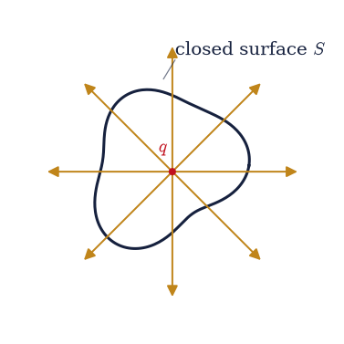
Fig. 201 Gauss’s law: a charge \(q\) inside an arbitrary closed surface \(S\) (here an irregular blob). The amber arrows are the field piercing the surface; the net flux \(\oint\mathbf E\cdot d\mathbf A\) counts the field lines leaving and equals \(q/\varepsilon_0\) no matter the surface’s shape or size.

q/ε₀ = 112.9409 V·m
  sphere R=0.05 m: flux/(q/ε₀) = 0.99998
  sphere R=0.10 m: flux/(q/ε₀) = 0.99998
  sphere R=0.20 m: flux/(q/ε₀) = 0.99998
  cube  L=0.10 m: flux/(q/ε₀) = 0.99999

Validation 1

✓  the flux through a sphere equals q/ε₀   [got 0.999979 vs expected 1 (rtol=0.01, atol=1e-09)]
✓  the flux equals q/ε₀ regardless of surface shape or size   [got 0.999988 vs expected 1 (rtol=0.01, atol=1e-09)]

True

Exercise 2 — The uniformly charged solid sphere (spherical class)

The first symmetry class is spherical. For a uniformly charged ball, the field must be radial and depend only on \(r\), so a concentric sphere is the natural Gaussian surface and Eq. 202 gives \(E\) immediately. Inside, the enclosed charge grows as \(r^3\) while the surface area grows as \(r^2\), so the field rises linearly; outside, the full charge is enclosed and the field falls as a point charge’s (Fig. 202):

\[ E(r) = \frac{kQ\,r}{R^3}\ (r<R), \qquad E(r) = \frac{kQ}{r^2}\ (r>R). \]

The ball below has radius \(R = 0.1\,\)m and carries \(Q = 1\,\)nC spread uniformly.

1. Evaluate the closed-form \(E(r)\) over the radial grid (the two branches joined with numpy.where at \(r=R\)).

2. Confirm the interior is \(\propto r\) and the exterior is \(\propto 1/r^2\) from the field ratios, and check continuity at \(r=R\) by comparing the inside and outside limits (the field is continuous, with a kink in slope).

3. Visualise \(E(r)\) and a faithful field map (Fig. 203, Fig. 204).

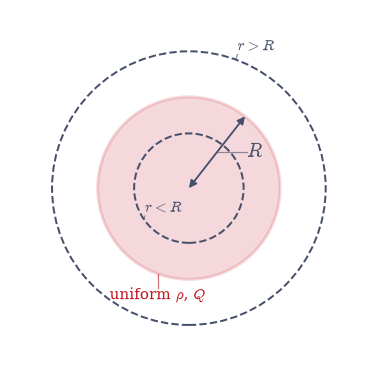
Fig. 202 The spherical Gaussian-surface construction for a uniformly charged ball of radius \(R\) and charge \(Q\) (shaded). A concentric Gaussian sphere drawn at \(r<R\) encloses only the fraction of charge within it (\(\propto r^3\)); one drawn at \(r>R\) encloses all of \(Q\). Symmetry makes \(\mathbf E\) radial and constant on each, so Gauss’s law gives \(E(r)\) directly.

interior E(0.05)/E(0.02) = 2.5000  (expect 2.5)
exterior E(0.2)/E(0.4)   = 4.0000  (expect 4)
continuity gap at r=R    = 8.988e-07 V/m

/tmp/ipykernel_3187/1968301667.py:21: RuntimeWarning: divide by zero encountered in divide
  return np.where(r < R_s, K * Q_s * r / R_s**3, K * Q_s / r**2)

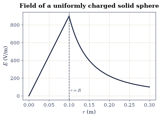
Fig. 203 The field of the uniformly charged solid sphere (\(R=0.1\,\)m, \(Q=1\,\)nC). Inside it rises linearly, \(E\propto r\) (enclosed charge \(\propto r^3\) beats area \(\propto r^2\)); outside it falls as \(1/r^2\), exactly a point charge of the full \(Q\). The two branches meet continuously at \(r=R\) (dashed), with only a kink in slope.

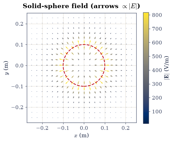
Fig. 204 Faithful field map of the solid sphere in a plane through its centre (ecp.draw.field_quiver): each arrow’s length and colour encode \(|\mathbf E|\). The arrows lengthen with \(r\) inside the sphere (dashed circle) and shorten outside it, the visual signature of the \(\propto r\) then \(\propto 1/r^2\) profile.

Validation 2

✓  the interior field is ∝ r   [got 2.5 vs expected 2.5 (rtol=0.001, atol=1e-09)]
✓  the exterior field is ∝ 1/r²   [got 4 vs expected 4 (rtol=0.001, atol=1e-09)]
✓  the field is continuous at the surface r=R   [got 8.98755e-07 vs expected 0 (rtol=1e-06, atol=0.001)]

True

Exercise 3 — The spherical shell and the shell theorem

A surface charge spread over a sphere produces no field at all inside it. Gauss’s law makes this almost obvious: any Gaussian sphere with \(r<R\) encloses zero charge, so its flux, and by symmetry the field, vanishes. Outside, the full charge is enclosed and the shell looks exactly like a point charge at its centre (Fig. 205). This is the electrostatic shell theorem, the twin of the gravitational one Newton needed for the Earth.

The shell below has radius \(R = 0.1\,\)m and carries \(Q = 1\,\)nC.

1. From Gauss’s law the interior field is exactly zero and the exterior is \(kQ/r^2\); confirm both from the closed-form field (a numpy.where split at \(r=R\)).

2. As an independent numerical check, approximate the shell by \(N=2000\) equal point charges on a Fibonacci-lattice sphere and superpose their fields (the point-charge superposition of §3.1): the interior field collapses to a tiny residual while the exterior matches \(kQ/r^2\).

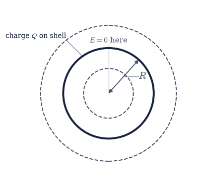
Fig. 205 The spherical shell (radius \(R\), charge \(Q\) on the surface, thick circle) with two Gaussian spheres: one inside (\(r<R\), enclosing no charge, so \(E=0\)) and one outside (\(r>R\), enclosing all of \(Q\), so \(E=kQ/r^2\)). The vanishing interior field is the shell theorem.

analytic interior field      = 0.000e+00 V/m
discrete interior |E|        = 3.457e-03 V/m  (3.85e-06 of surface field)
discrete exterior |E|        = 1.4380e+02 V/m  (expect 1.4380e+02)

Validation 3

✓  the field vanishes inside a spherical shell (shell theorem)   [got 0 vs expected 0 (rtol=1e-06, atol=1e-09)]
✓  the superposed shell's interior field is negligible vs its surface field   [got 3.84674e-06 vs expected 0 (rtol=1e-06, atol=0.01)]
✓  outside, the shell acts as a point charge kQ/r²   [got 143.8 vs expected 143.801 (rtol=0.01, atol=1e-09)]

True

Exercise 4 — The infinite line charge (cylindrical class)

The second class is cylindrical. A uniformly charged infinite line has a field that points radially outward (in the plane perpendicular to the line) and depends only on the perpendicular distance \(r\), so the Gaussian surface is a coaxial cylinder (Fig. 206). Its curved wall has area \(2\pi r L\) and the flat caps contribute nothing, so Eq. 202 gives

\[ E(r) = \frac{\lambda}{2\pi\varepsilon_0\,r}. \]

The falloff is \(1/r\), slower than a point charge’s \(1/r^2\): a line reaches farther because its charge is spread along a whole dimension.

The line below carries \(\lambda = 1\,\)nC/m.

1. Evaluate \(E=\lambda/(2\pi\varepsilon_0 r)\) over the radial grid and confirm the \(1/r\) falloff from the ratio \(E(0.1)/E(0.2)\).

2. Draw a faithful map of the radial field in the plane perpendicular to the line (Fig. 207).

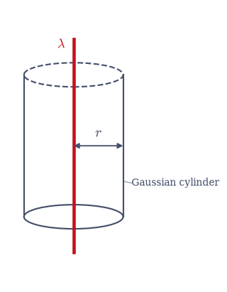
Fig. 206 The cylindrical Gaussian surface for an infinite line charge of density \(\lambda\) (vertical, red): a coaxial cylinder of radius \(r\) and length \(L\). The field is radial and constant on the curved wall (area \(2\pi r L\)) and parallel to the flat caps (zero flux there), so Gauss’s law gives \(E=\lambda/2\pi\varepsilon_0 r\).

line-charge E(0.1)/E(0.2) = 2.0000  (expect 2 for 1/r)

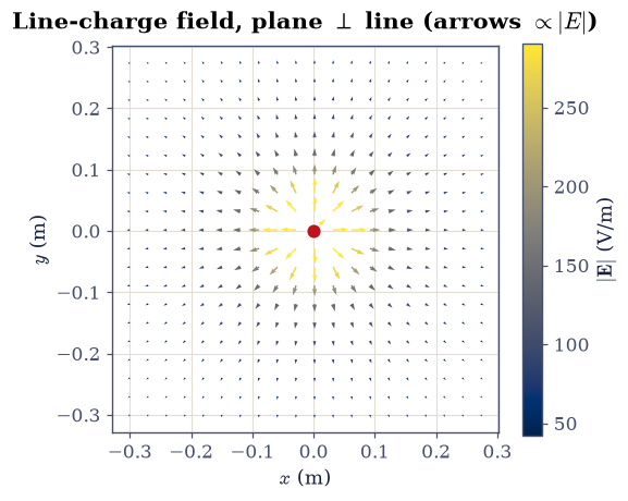
Fig. 207 Faithful field map of the infinite line charge in the plane perpendicular to it (ecp.draw.field_quiver): arrow length and colour encode \(|\mathbf E|\propto 1/r\). The arrows point radially outward and shrink with distance, but more gently than a point charge’s \(1/r^2\).

Validation 4

✓  the line-charge field falls as 1/r   [got 2 vs expected 2 (rtol=0.001, atol=1e-09)]

True

Exercise 5 — The infinite sheet and the parallel-plate capacitor (planar class)

The third class is planar. An infinite sheet of charge has a field that points straight away from it and, remarkably, does not weaken with distance. A pillbox Gaussian surface straddling the sheet (Fig. 208) catches flux \(EA\) through each of its two faces and encloses charge \(\sigma A\), so

\[ 2EA = \frac{\sigma A}{\varepsilon_0} \;\Longrightarrow\; E = \frac{\sigma}{2\varepsilon_0}, \]

independent of distance. That a field can be perfectly uniform is genuinely surprising on first sight; it is the planar geometry’s answer to the \(1/r^2\) and \(1/r\) of the other classes. Two oppositely charged sheets then superpose: their fields add to \(\sigma/\varepsilon_0\) in the gap and cancel to zero outside, which is the ideal parallel-plate capacitor.

The sheets below each carry \(\sigma = 1\,\)nC/m².

1. Confirm the uniformity by measurement, not by restating the formula: evaluate the on-axis field of a large finite disk (radius \(10\,\)m, far larger than the distances probed) at \(z = 0.01\) and \(0.02\,\)m via the closed form \(E(z)=\sigma/2\varepsilon_0\,(1-z/\sqrt{z^2+R^2})\), and show the two values agree with each other and with the infinite-sheet \(\sigma/2\varepsilon_0\).

2. Obtain the two-sheet capacitor field by superposing the oppositely charged sheets (numpy.where for the between/outside regions), and confirm \(\sigma/\varepsilon_0\) between the plates and zero outside (Fig. 209).

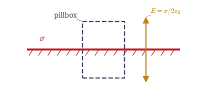
Fig. 208 The pillbox Gaussian surface for an infinite charged sheet (density \(\sigma\), horizontal). The box straddles the sheet; flux leaves through its two faces (area \(A\) each) and the field is uniform on both, while the side walls catch none. Gauss’s law gives the distance-independent \(E=\sigma/2\varepsilon_0\), drawn as equal arrows above and below.

disk (R=10 m) E at z=0.01, 0.02 m: 56.4140, 56.3575 V/m (ratio 1.001002; infinite sheet 56.4705 V/m)
capacitor: between = 112.9409 V/m (= σ/ε₀ = 112.9409), outside = 0.0000 V/m

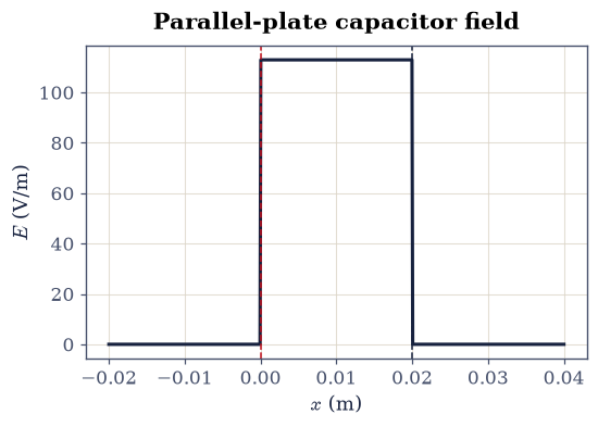
Fig. 209 The parallel-plate capacitor field across \(x\) for sheets \(+\sigma\) at \(x=0\) and \(-\sigma\) at \(x=d\) (dashed). The two uniform single-sheet fields superpose to a constant \(\sigma/\varepsilon_0\) in the gap and cancel to zero outside, the textbook capacitor.

Validation 5

✓  a large sheet's near field is uniform: measured on a 10 m disk at two distances   [got 1.001 vs expected 1 (rtol=0.01, atol=1e-09)]
✓  and it matches the infinite-sheet value σ/2ε₀   [got 56.414 vs expected 56.4705 (rtol=0.005, atol=1e-09)]
✓  two opposite sheets give σ/ε₀ between them   [got 112.941 vs expected 112.941 (rtol=1e-09, atol=1e-09)]
✓  the capacitor field is zero outside the plates   [got 0 vs expected 0 (rtol=1e-06, atol=1e-09)]

True

Exercise 6 — The charged slab (student)

A slab of finite thickness combines the planar symmetry with interior structure: inside, only the charge between the centre plane and the field point is enclosed, so the field grows linearly; outside, the whole column is enclosed and the field saturates, just like an infinite sheet (Fig. 210). For a slab of half-thickness \(a\) and uniform density \(\rho\), a pillbox argument gives

\[ E(x) = \frac{\rho\,x}{\varepsilon_0}\ (|x|<a), \qquad E(x) = \frac{\rho\,a}{\varepsilon_0}\ (|x|>a). \]

The slab below has uniform density \(\rho = 10^{-6}\,\)C/m³ and half-thickness \(a = 0.05\,\)m.

1. Using Gauss’s law with a pillbox straddling the mid-plane, write \(E(x)\) for \(|x|<a\) and \(|x|>a\) and evaluate it over the grid with numpy.where for the inside/outside branches.

2. Confirm the interior grows \(\propto x\) and the exterior saturates at the constant \(\rho a/\varepsilon_0\), and plot the ramp-then-plateau profile (Fig. 211).

/tmp/ipykernel_3187/2471179576.py:15: UserWarning: linestyle is redundantly defined by the 'linestyle' keyword argument and the fmt string "-" (-> linestyle='-'). The keyword argument will take precedence.
  ax.plot([0, 0], [-1.2, 1.2], "-", color=draw.SOFT, lw=1.0, ls=":")

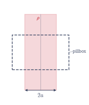
Fig. 210 The charged slab of half-thickness \(a\) and uniform density \(\rho\) (shaded band), with a pillbox straddling the mid-plane \(x=0\). The enclosed charge grows with the pillbox half-width while it lies inside the slab and then stops growing once the box pokes out, giving \(E\propto x\) inside and a constant \(\rho a/\varepsilon_0\) outside.

interior E(a/2)/E(a/4) = 2.0000  (expect 2)
exterior E = 5647.0453 V/m  (expect ρa/ε₀ = 5647.0453)

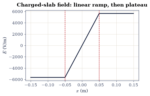
Fig. 211 The slab field \(E(x)\) across the slab (\(\rho=10^{-6}\,\)C/m³, \(a=0.05\,\)m; slab edges dashed). The field ramps linearly through the interior, \(E\propto x\), then saturates at the constant \(\rho a/\varepsilon_0\) once outside, where the slab looks like a sheet of surface density \(\sigma=2\rho a\).

Validation 6

✓  the slab field grows linearly inside (∝ x)   [got 2 vs expected 2 (rtol=0.001, atol=1e-09)]
✓  the slab field saturates outside at ρa/ε₀   [got 5647.05 vs expected 5647.05 (rtol=0.001, atol=1e-09)]

True

Exercise 7 — The differential form: ∇·E = ρ/ε₀ numerically

Shrinking Gauss’s law to a point gives the local field equation Eq. 203, \(\nabla\cdot\mathbf E = \rho/\varepsilon_0\). We can read it off a grid directly: the divergence is a sum of central differences of the field components, the same stencils as §0.3, evaluated here with numpy.gradient (Fig. 212). For the uniformly charged sphere of Exercise 2 the interior field is \(\mathbf E=(kQ/R^3)\,\mathbf r\), whose divergence is the constant \(3kQ/R^3=\rho/\varepsilon_0\); outside, the field is source-free.

1. Build the solid-sphere field of Exercise 2 (\(R=0.1\,\)m, \(Q=1\,\)nC) as a vector field on an \(81^3\) grid over \([-0.2, 0.2]^3\,\)m.

2. Compute \(\nabla\cdot\mathbf E = \partial_x E_x + \partial_y E_y + \partial_z E_z\) with numpy.gradient.

3. Confirm it equals \(\rho/\varepsilon_0\) in the interior (well inside, away from the surface kink) and is \(\approx 0\) in the empty space outside.

This local statement, field tied to source at every point, is the first field equation of the course. It is the sense in which electrodynamics, in Landau and Lifshitz’s framing, is the exemplar of a classical field theory: the physics lives in differential equations the field obeys everywhere, not in forces between distant particles.

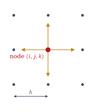
Fig. 212 The central-difference stencil behind the numerical divergence: at a grid node (red), each component’s derivative is formed from its two neighbours a step \(h\) apart along that axis (here the in-plane \(x\) and \(y\) neighbours of the \(81^3\) grid). Summing \(\partial_x E_x+\partial_y E_y+\partial_z E_z\) at every node gives \(\nabla\cdot\mathbf E\).

⟨∇·E⟩ inside / (ρ/ε₀) = 1.00000  (expect 1)
max|∇·E| outside / (ρ/ε₀) = 1.55e-03  (expect ≈ 0)

Validation 7

✓  ∇·E = ρ/ε₀ inside the charged sphere (the differential field equation)   [got 1 vs expected 1 (rtol=0.01, atol=1e-09)]
✓  the field is divergence-free in empty space

True

Exercise 8 — The gravitational parallel: through the Earth (student)

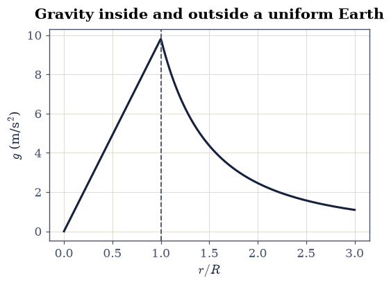
Because Gauss’s law needs only the inverse-square form, the spherical results transfer to gravity unchanged. Model the Earth as a uniform sphere of mass \(M\) and radius \(R\). By the gravitational Gauss law Eq. 204 (the field points inward, the honest sign of attraction; there is no negative mass and so no shielding), the field inside grows linearly, \(g(r) = GM\,r/R^3\), exactly mirroring the charged sphere of Exercise 2 (Fig. 213). A mass dropped into a tunnel through the centre therefore feels a restoring force \(\propto -r\), the signature of simple harmonic motion.

The Earth below is uniform, with \(M = 5.972\times10^{24}\,\)kg, \(R = 6.371\times10^{6}\,\)m, and \(G = 6.674\times10^{-11}\,\)N·m²/kg², and a mass is released from rest at the surface inside a frictionless tunnel through the centre.

1. Write tunnel_rhs(t, y), the state derivative of that motion for \(\mathbf y = [x, v]\): the linear interior field makes it \([\,v,\ -\omega^2 x\,]\) with \(\omega^2 = GM/R^3\). Write this one yourself — the implementation is the lesson.

2. Integrate the motion with scipy.integrate.solve_ivp (DOP853, with a zero-crossing event to time the swing), measure the oscillation period, and compare it to the SHM prediction \(T = 2\pi\sqrt{R^3/GM}\).

3. Note the small delight that this equals the period of a surface-skimming orbit (both are \(2\pi\sqrt{R^3/GM}\)), a callback to the orbital periods of §1.4 and §2.4.

4. Plot \(g(r)\) inside and outside the Earth (Fig. 214).

/tmp/ipykernel_3187/2511264104.py:10: UserWarning: linestyle is redundantly defined by the 'linestyle' keyword argument and the fmt string "-" (-> linestyle='-'). The keyword argument will take precedence.
  ax.plot([0, 0], [-1.0, 1.0], "-", color=draw.SOFT, lw=1.0, ls=":")

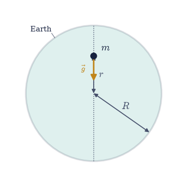
Fig. 213 The through-the-Earth problem: a uniform Earth of radius \(R\) (shaded) with a frictionless tunnel through the centre (dotted). A mass \(m\) at radius \(r\) feels the gravity of only the enclosed sphere, \(g(r)=GM r/R^3\), pointing inward (amber). The linear restoring field makes the motion simple harmonic.

measured period = 5060.91 s = 84.3 min
SHM prediction  = 5060.91 s = 84.3 min
(equals the surface-orbit period 2π√(R³/GM) — same √(R³/GM))

Fig. 214 The gravitational field strength \(g(r)\) for a uniform Earth (surface dashed). Inside it rises linearly, \(g=GM r/R^3\) (the source of the simple-harmonic tunnel motion); outside it falls as \(GM/r^2\). This is the exact gravitational mirror of the charged solid sphere in Fig. 203.

Validation 8

✓  the through-Earth oscillation is SHM with period 2π√(R³/GM)   [got 5060.91 vs expected 5060.91 (rtol=0.001, atol=1e-09)]

True

Exercise 9 — When Gauss’s law is, and isn’t, enough

Gauss’s law is always true, but it only gives the field when symmetry pins the field’s direction and magnitude on a Gaussian surface. Drop the symmetry and the law still holds as a bookkeeping identity, the flux still equals \(Q_{\text{enc}}/\varepsilon_0\), but it can no longer be inverted for \(\mathbf E\): one scalar equation cannot determine a vector field that varies over the surface (Fig. 215). That is exactly the situation that forces us to solve Poisson’s equation directly, the boundary-value problem of §3.4.

Two unequal charges sit below, \(q_1 = 1\,\)nC at \((-0.1, 0, 0)\) and \(q_2 = 3\,\)nC at \((0.15, 0, 0)\,\)m. The distribution has no symmetry that fixes the field, yet the flux through any enclosing surface must still be \((q_1+q_2)/\varepsilon_0\).

1. Verify this numerically with the Setup’s flux_through_sphere — the same \((\theta,\varphi)\) trapezoid as in Exercise 1, now fed two source charges — on a sphere of radius \(0.5\,\)m enclosing both.

2. Note that the same calculation gives us no way to read off \(\mathbf E\) pointwise — the gateway to §3.4.

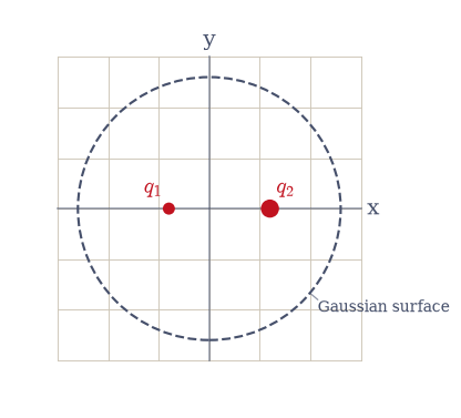
Fig. 215 An asymmetric pair: unequal charges \(q_1\) and \(q_2\) enclosed by a Gaussian sphere (dashed). Gauss’s law still fixes the total flux at \((q_1+q_2)/\varepsilon_0\), but with no symmetry to make \(\mathbf E\) constant on the surface it cannot be solved for the field, which is what motivates Poisson’s equation in §3.4.

flux/(Q_enc/ε₀) for the asymmetric pair = 0.99998  (expect 1)

Validation 9

✓  Gauss's law holds even when it cannot give the field by symmetry alone   [got 0.999981 vs expected 1 (rtol=0.01, atol=1e-09)]

True

Notebook summary

• Flux \(\oint\mathbf E\cdot d\mathbf A=q/\varepsilon_0\) for any enclosing surface (sphere and cube agreeing to \(\sim10^{-4}\)), independent of shape or size.

• The three symmetry classes solved from Gauss’s law: the uniformly charged ball (\(E\propto r\) inside, \(1/r^2\) outside, continuous at \(R\)), the shell (zero interior field, the shell theorem), the infinite line (\(E\propto1/r\)), the sheet and capacitor (\(E\) constant), and the slab (\(E\propto x\) inside).

• The differential form \(\nabla\cdot\mathbf E=\rho/\varepsilon_0\) confirmed numerically (numpy.gradient divergence); the gravitational parallel (simple-harmonic fall through the Earth); and where symmetry fails, motivating Poisson’s equation in §3.4.

Outlook

• Conductors and Gauss’s law. Just outside a conductor the field is \(\sigma/\varepsilon_0\) (a pillbox with one face inside, where \(\mathbf E=0\)), all excess charge lives on the outer surface, and a hollow conductor shields its interior, the Faraday cage. These follow directly from the law and set up the boundary-value problems of §3.4.

• The gravitational shell theorem. Newton needed exactly the result of Exercise 3 to treat the Earth and Moon as point masses; the gradient of \(g\) across a body is the tidal field.

• Why \(1/r^2\) exactly. Gauss’s law is the statement that field lines are conserved in three dimensions; the \(1/r^2\) is nothing but the \(r^2\) surface area of a sphere. In \(d\) dimensions the law would give \(E\propto 1/r^{\,d-1}\), a clean way to see what is special about living in three.

• Forward links. Poisson’s equation and the boundary-value problem (§3.4); the full set of field equations (Maxwell, §3.8); and the covariant field-equation viewpoint of the relativistic capstone (§3.12), where \(\nabla\cdot\mathbf E=\rho/ \varepsilon_0\) becomes one component of a single four-dimensional law.

References

[Gri17]

David J. Griffiths. Introduction to Electrodynamics. Cambridge University Press, 4 edition, 2017.

[LL80]

L. D. Landau and E. M. Lifshitz. The Classical Theory of Fields. Volume 2 of Course of Theoretical Physics. Butterworth-Heinemann, 4 edition, 1980.

[Nol16]

Wolfgang Nolting. Theoretical Physics 3: Electrodynamics. Springer, 2016.

Take this notebook with you

Use the download button (↓) in the toolbar above to save this notebook and run it yourself. The published notebooks ship without worked solutions; if you would like the reference solutions — to teach from or to check your own work — get in touch: hello@ramador.me.