6.7 Time Evolution and the Schrödinger Equation

Elementary Computational Physics

Volume VI — Quantum Mechanics Notebook 6.7

Setting the state in motion. The last postulate said the state evolves by the Schrödinger equation; here we solve it. The Hamiltonian generates a unitary flow, U(t)=e^{−iHt/ℏ}, under which energy eigenstates merely turn their phase and everything else beats between them. In the two-state system the motion is visible: a spin precesses, a driven qubit oscillates between its levels — the dynamics behind magnetic resonance, atomic clocks, and quantum gates.

Level · advanced   •   Est. · 160–195 min

Raymond Amador v1.4.0  ·  2026-07-31  ·  CC BY 4.0 (text) / MIT (code)

Notebook overview

The fifth postulate (§6.5) was stated and then set aside: between measurements, the state evolves by the Schrödinger equation \(i\hbar\,\partial_t|\psi\rangle=H|\psi\rangle\). This notebook delivers on that deferral. It solves the equation, and in doing so reveals the structure of all quantum dynamics — which turns out to be simpler, and more beautiful, than the equation first suggests.

The solution is a single operator. For a time-independent Hamiltonian the state at time \(t\) is \(|\psi(t)\rangle=U(t)|\psi(0)\rangle\) with the time-evolution operator \(U(t)=e^{-iHt/\hbar}\) — the exponential map of §6.2, the prime function-of-operator of §6.3. Because \(H\) is Hermitian, \(U(t)\) is unitary, so the norm and hence total probability are conserved, exactly as a state evolution must guarantee. And in the Hamiltonian’s own eigenbasis the flow is trivial: each energy eigenstate merely rotates its phase, \(|n\rangle\to e^{-iE_nt/\hbar}|n\rangle\). An energy eigenstate is therefore stationary — every probability frozen — and a general state is a sum of such phases beating against one another at the Bohr frequencies \((E_n-E_m)/\hbar\). All dynamics is this interference of phases, which is why the central task of quantum mechanics is to find the energy eigenstates: once \(H\) is diagonalized, time evolution is free.

In the two-state system the abstract flow becomes visible motion. A spin in a magnetic field precesses — its expectation vector rotates about the field at the Larmor frequency, a classical motion emerging from unitary evolution — and a driven two-level system undergoes Rabi oscillations, cycling between its levels. These are not toys: they are the physics of nuclear magnetic resonance and MRI, of atomic clocks, and of the gates that drive a qubit in a quantum computer. We close with Ehrenfest’s theorem, \(d\langle A\rangle/dt=(i/\hbar)\langle[H,A]\rangle\), which says exactly which quantities are conserved — those commuting with \(H\) (§6.6) — and bridges back to the Poisson brackets of Volume II.

As in every Volume VI notebook, each exercise opens with a crystal-clear statement and enumerated parts, each naming the exact operation — scipy.linalg.expm for \(U(t)\) alongside the transparent spectral construction \(U=\sum_n e^{-iE_nt/\hbar}|n\rangle\langle n|\), numpy.linalg.eigh for the energy eigenbasis, and numpy.vdot for the expectation traces \(\langle A\rangle(t)\).

How to read the checks. Each exercise closes with a validate call: \(U(t)\) solving \(i\hbar \dot U=HU\) and unitary; an energy eigenstate acquiring only a phase; a superposition beating at the Bohr frequency; the Larmor traces \(\langle S_x\rangle=\tfrac12\cos\omega t\), \(\langle S_y\rangle= -\tfrac12\sin\omega t\); resonant Rabi \(P_e=\sin^2(\Omega t/2)\) and its off-resonant shrinking; and Ehrenfest’s theorem with \(\langle S_z\rangle\) conserved. A ✓ is strong evidence; a ✗ is a prompt to locate the discrepancy.

Conventions and scope. We set \(\hbar=1\) (restored in formulas where it clarifies). The Pauli matrices are those of §6.6, with spin operators \(S=\tfrac12\boldsymbol\sigma\). The Larmor Hamiltonian is \(H=-\gamma\,\mathbf B\cdot\mathbf S\); the driven two-level Hamiltonian is \(H=\tfrac{\delta}{2} \sigma_z+\tfrac{\Omega}{2}\sigma_x\) with detuning \(\delta\) and coupling \(\Omega\). The Bloch-sphere geometry of precession is §6.8; continuous-system dynamics (wave packets) is §6.10–§6.13; driven transitions in many levels is §6.24. See Sakurai & Napolitano (§2.1, §2.3); the Feynman Lectures Vol. III; and Notebooks §6.2 (the exponential map), §6.3 (functions of operators), §6.5 (the postulate), §6.6 (commutators, conservation), and Volume II (Poisson brackets).

Theory in brief

The Schrödinger equation and the time-evolution operator

The dynamics postulate is \(i\hbar\,\partial_t|\psi\rangle=H|\psi\rangle\), with \(H\) the Hamiltonian (the energy observable, Hermitian). For time-independent \(H\) the solution is

(527)\[|\psi(t)\rangle=U(t)|\psi(0)\rangle,\qquad U(t)=e^{-iHt/\hbar},\qquad i\hbar\,\dot U=HU,\quad U^{\dagger}U=I .\]

\(U(t)\) is the exponential map of §6.2 / the function-of-operator of §6.3, and it is unitary (because \(H\) is Hermitian), so the norm and total probability are conserved.

The energy eigenbasis and stationary states

In the eigenbasis of \(H\), with \(H|n\rangle=E_n|n\rangle\), the operator is \(U(t)=\sum_n e^{-iE_nt/\hbar} |n\rangle\langle n|\) (§6.3). An energy eigenstate evolves by a mere phase,

(528)\[|\psi(t)\rangle=e^{-iE_nt/\hbar}|n\rangle\ \text{(stationary)},\qquad |\psi\rangle=\sum_n c_n|n\rangle\ \to\ \sum_n c_n e^{-iE_nt/\hbar}|n\rangle ,\]

so all its probabilities are time-independent. A general state’s amplitudes beat at the Bohr frequencies \((E_n-E_m)/\hbar\) — all dynamics is this interference of phases. This is why diagonalizing \(H\) is the central task: once done, time evolution is free.

Spin precession (Larmor)

A spin in a uniform field has \(H=-\gamma\,\mathbf B\cdot\mathbf S\); for \(\mathbf B\) along \(z\), \(H=-\tfrac{\omega}{2}\sigma_z\) with \(\omega=\gamma B\) the Larmor frequency. A spin started along \(x\) precesses,

(529)\[\langle S_x\rangle=\tfrac{\hbar}{2}\cos\omega t,\quad \langle S_y\rangle=-\tfrac{\hbar}{2}\sin\omega t,\quad \langle S_z\rangle\ \text{conserved} ,\]

a classical precession of the spin vector about the field, emerging from unitary evolution (the physics of NMR/MRI).

Rabi oscillations

A two-level system with detuning \(\delta\) driven by a coupling \(\Omega\) has \(H=\tfrac{\delta}{2} \sigma_z+\tfrac{\Omega}{2}\sigma_x\). Started in the lower level, the upper-level population is

(530)\[\text{on resonance }(\delta=0):\ P_e(t)=\sin^2\tfrac{\Omega t}{2};\qquad \text{off resonance: }P_e^{\max}=\frac{\Omega^2}{\Omega^2+\delta^2}\ \text{at}\ \Omega_R=\sqrt{\Omega^2+\delta^2} .\]

On resonance the cycling is complete (a \(\pi\)-pulse, \(\Omega t=\pi\), flips the state); off resonance it is faster but shallower. Sakurai & Napolitano (§5.5) derive Rabi’s formula in full; the Feynman Lectures Vol. III reach the same physics through the ammonia maser. This is how a qubit is driven — NMR pulses, laser excitation, single-qubit gates.

Ehrenfest’s theorem and conservation

For an observable \(A\) without explicit time dependence, one line of calculus suffices: differentiate \(\langle\psi|A|\psi\rangle\) and let the Schrödinger equation supply \(\partial_t|\psi\rangle\) and its adjoint (Griffiths, Ch. 3, records the general statement),

(531)\[\frac{d\langle A\rangle}{dt}=\frac{i}{\hbar}\langle[H,A]\rangle ,\]

so an observable that commutes with \(H\) is conserved (and energy always is). The commutator \([H,\cdot]\) plays the role of the classical Poisson bracket \(\{H,\cdot\}\) of Volume II — canonical quantization is \(\{\cdot,\cdot\}\to\tfrac{1}{i\hbar}[\cdot,\cdot]\).

Setup

The data are the series palette, the convention \(\hbar=1\), and the Pauli matrices of §6.6 with their spin operators \(S=\tfrac12\boldsymbol\sigma\) — the fixed matrices every Hamiltonian below is written in terms of. The two instruments are expectation_value, a one-line wrapper on numpy.vdot for \(\langle\psi|A|\psi\rangle\) (§6.5), and expectation_trace, which assembles the time-resolved signal \(\langle A\rangle(t)\) by sampling the evolution on a grid of times. The propagator itself — the thing this notebook is named for — is not here: you write evolve in Exercise 1, and expectation_trace picks up the one you wrote.

The Setup below holds this notebook’s data and instruments — nothing you are asked to build. It is collapsed so the building stays yours; expand it whenever you want the details.

Show code cell source

Hide code cell source

import matplotlib.pyplot as plt
import numpy as np
from matplotlib.animation import FuncAnimation
from scipy.linalg import expm

from ecp import draw, validate
from ecp.animate import show

# data: the series palette
ACCENT, INK, SOFT = draw.ACCENT, draw.INK, draw.SOFT

# data: conventions. ℏ=1. The Pauli matrices (§6.6) and spin operators S=½σ; states are unit
# complex vectors. Time evolution uses the spectral construction U=Σe^{−iE_n t}|n⟩⟨n| from
# numpy.linalg.eigh (transparent and efficient), cross-checked against scipy.linalg.expm; expectation
# values use numpy.vdot (conjugate-first, §6.1).

SIGMA_X = np.array([[0, 1], [1, 0]], dtype=complex)
SIGMA_Y = np.array([[0, -1j], [1j, 0]], dtype=complex)
SIGMA_Z = np.array([[1, 0], [0, -1]], dtype=complex)
S_X, S_Y, S_Z = SIGMA_X / 2, SIGMA_Y / 2, SIGMA_Z / 2


# instrument: the reading device, a single ``numpy.vdot`` — every exercise here measures
# *with* it, never about it; the Born-rule content behind it is the lesson of §6.5, not of
# this notebook.
def expectation_value(A, psi):
    """The expectation value $\\langle A\\rangle=\\langle\\psi|A|\\psi\\rangle$ (§6.5), via ``numpy.vdot``.

    Real because $A$ is Hermitian (``numpy.vdot(psi, A @ psi).real``).
    """
    return np.vdot(psi, A @ psi).real


# instrument: signal assembly — looping a grid of times and reading ⟨A⟩ off each state is
# bookkeeping, not physics. It calls whatever ``evolve`` is bound to when it runs: the one you
# write in Exercise 1 (Python looks the name up at call time, not at definition time).
def expectation_trace(H, psi0, A, times):
    """The trace $\\langle A\\rangle(t)$ of an observable as the state evolves {eq}`eq-stationary`.

    Evolves ``psi0`` to each time in ``times`` with the ``evolve`` of Exercise 1 and returns the array of
    expectation values $\\langle\\psi(t)|A|\\psi(t)\\rangle$ — the laboratory's time-resolved signal.

    Parameters
    ----------
    H : numpy.ndarray
        The Hamiltonian.
    psi0 : numpy.ndarray
        The initial state.
    A : numpy.ndarray
        The observable to track.
    times : array_like
        The times at which to sample.

    Returns
    -------
    numpy.ndarray
        $\\langle A\\rangle(t)$ at each time.
    """
    return np.array([expectation_value(A, evolve(H, psi0, t)) for t in times])

Exercise 1 — The time-evolution operator

For a time-independent Hamiltonian the Schrödinger equation is solved once and for all by the time-evolution operator \(U(t)=e^{-iHt}\) (with \(\hbar=1\)) — the dynamics postulate, solved Eq. 527. Two constructions give the same operator. The matrix exponential scipy.linalg.expm(-1j*H*t) computes it directly; the spectral construction builds it out of the energy eigenbasis, \(U(t)=\sum_n e^{-iE_nt}|n\rangle\langle n|\), which is what the state actually does — diagonalize \(H\) with numpy.linalg.eigh, expand the initial state in the eigenvectors as \(c_n=\langle n|\psi_0\rangle\), turn each component’s phase by \(e^{-iE_nt}\), and transform back. That second route is the one worth writing: it exposes the physics (evolution is a set of rotating phases) and it is far cheaper when many times are wanted, which is why every later exercise here runs on it. The three things it must satisfy are the equation itself, \(i\dot U=HU\); unitarity, \(U^{\dagger}U=I\); and the conservation of probability that unitarity guarantees. The specimen is a random Hermitian \(H\) on \(\mathbb C^3\) evaluated at \(t=0.8\).

1. Write evolve(H, psi0, t), returning \(|\psi(t)\rangle\) by the spectral construction. Write this one yourself — the implementation is the lesson.

2. Build \(U(t)\) with scipy.linalg.expm(-1j*H*t) and, independently, as \(\sum_n e^{-iE_nt}|n\rangle\langle n|\) from numpy.linalg.eigh (energies and eigenvectors); confirm the two agree with numpy.allclose.

3. Verify \(i\dot U=HU\) by approximating \(\dot U\) with a centered finite difference \([U(t+dt)-U(t-dt)]/(2dt)\) and comparing \(i\dot U\) to H @ U.

4. Verify \(U^{\dagger}U=I\) (U.conj().T @ U equals numpy.eye).

5. Evolve a state with the evolve you wrote and confirm its norm is preserved.

expm vs spectral Σe^(−iE_nt)|n⟩⟨n|:  agree = True
iU̇ = HU:  max|iU̇ − HU| = 2.8e-10
U†U = I:  max|U†U − I| = 7.8e-16
‖ψ(t)‖ = 1.0000000000   (probability conserved)

Validation 1

✓  U(t)=e^{−iHt} solves the Schrödinger equation iU̇=HU and is unitary (norm and probability conserved)   [max|Δ| = 2.75366e-10 (rtol=1e-06, atol=1e-05)]

True

Exercise 2 — Stationary states

Show why energy eigenstates are special: an eigenstate of \(H\) evolves by a pure phase, so every observable’s probabilities in it are frozen in time — a stationary state Eq. 528.

1. Diagonalize \(H\) with numpy.linalg.eigh and take an eigenstate \(|n\rangle\) (a column of the eigenvector matrix) with energy \(E_n\).

2. Evolve it to several times with the evolve you wrote in Exercise 1.

3. Confirm \(|\psi(t)\rangle=e^{-iE_nt}|n\rangle\) — only a phase — by checking \(|\langle n| \psi(t)\rangle|=1\) at every time (numpy.abs(numpy.vdot(...))).

4. Confirm the expectation of an arbitrary observable is time-independent in this state. Frame: this is why “find the energy eigenstates” is the central task — once diagonalized, evolution is a set of phases.

|⟨n|ψ(t)⟩| over time: min = 1.000000, max = 1.000000   (all 1: stationary)
|ψ(t)⟩ = e^(−iE_n t)|n⟩ (a pure phase): True
⟨A⟩(t) in the eigenstate: spread = 1.9e-15   (constant)

Validation 2

✓  an energy eigenstate is stationary — it acquires only a phase e^{−iE_nt}, so |⟨n|ψ(t)⟩|=1 and every probability is frozen   [max|Δ| = 8.88178e-16 (rtol=1e-12, atol=1e-09)]

True

Exercise 3 — Beats: the evolution of a superposition

Evolve an equal superposition of two energy eigenstates and show that an observable not diagonal in the energy basis oscillates at the Bohr frequency \((E_2-E_1)/\hbar\) — the beating of energy phases that is all of quantum dynamics Eq. 528.

1. Take a Hamiltonian with known energies (e.g. \(H=\mathrm{diag}(E_1,E_2)\)) and form the superposition \(|\psi\rangle=(|1\rangle+|2\rangle)/\sqrt2\).

2. Evolve it with your Exercise 1 evolve over a grid of times (numpy.linspace).

3. Compute \(\langle A\rangle(t)\) with the Setup’s expectation_trace — which evolves with that same evolve — for an observable off-diagonal in the energy basis (e.g. \(\sigma_x\)).

4. Identify the oscillation frequency as \((E_2-E_1)/\hbar\) — read it off the period, or confirm \(\langle\sigma_x\rangle(t)=\cos [(E_2-E_1)t]\). All dynamics is the interference of energy-eigenstate phases.

⟨σx⟩(t) oscillates at the Bohr frequency (E2−E1)/ℏ = 2.0:  True
  period = 2π/(E2−E1) = 3.1416

Validation 3

✓  a superposition of two energy eigenstates beats: an off-diagonal observable oscillates at the Bohr frequency (E2−E1)/ℏ   [max|Δ| = 1.80411e-15 (rtol=1e-10, atol=1e-09)]

True

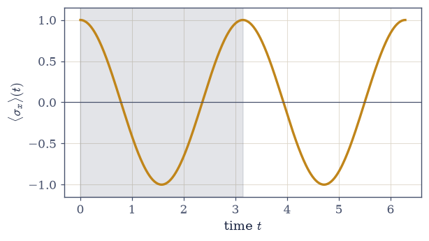
Fig. 521 All dynamics is the beating of energy phases. An equal superposition of two energy eigenstates, \((|1\rangle+|2\rangle)/\sqrt2\), is evolved; the expectation \(\langle\sigma_x\rangle(t)\) of an observable off-diagonal in the energy basis (amber) oscillates as \(\cos[(E_2-E_1)t]\), exactly at the Bohr frequency \((E_2-E_1)/\hbar\) (one period marked). Each eigenstate only turns its phase \(e^{-iE_nt}\) — stationary on its own — but the two phases run at different rates, and their interference is the entire visible motion. This is why diagonalizing \(H\) solves the dynamics: every signal a system produces is a sum of these beats.

Exercise 4 — Spin precession (Larmor)

A spin in a magnetic field along \(z\), started along \(x\), is evolved under the Larmor Hamiltonian \(H=-\tfrac{\omega}{2}\sigma_z\) (i.e. \(-\gamma\mathbf B\cdot\mathbf S\) for \(\mathbf B\parallel \hat z\)). Find \(\langle S_x\rangle(t)\), \(\langle S_y\rangle(t)\), \(\langle S_z\rangle(t)\) and show the spin vector precesses about the field at the Larmor frequency \(\omega\) Eq. 529. The rotation looks entirely classical, yet it emerges from unitary evolution alone — this is the physics of NMR.

1. Build \(H=-\tfrac{\omega}{2}\,\)SIGMA_Z.

2. Start in \(|{+}x\rangle=\)numpy.array( [1,1])/numpy.sqrt(2).

3. Compute the three traces over a grid of times with the Setup’s expectation_trace, which evolves the state with the evolve you wrote in Exercise 1, for S_X, S_Y, S_Z.

4. Confirm \(\langle S_x\rangle=\tfrac12\cos \omega t\), \(\langle S_y\rangle=-\tfrac12\sin\omega t\), and \(\langle S_z\rangle\) is conserved (zero) — a classical precession of the spin vector about the field.

⟨Sx⟩ = ½cos(ωt):  True
⟨Sy⟩ = −½sin(ωt): True
⟨Sz⟩ conserved (spread = 0.0e+00, value 0.00)

Validation 4

✓  a spin precesses about the field at the Larmor frequency: ⟨Sx⟩=½cos(ωt), ⟨Sy⟩=−½sin(ωt)   [max|Δ| = 2.22045e-16 (rtol=1e-09, atol=1e-09)]
✓  the component along the field, ⟨Sz⟩, is conserved during precession (it commutes with H)   [got 0 vs expected 0 (rtol=1e-06, atol=1e-12)]

True

Once Loop Reflect

Fig. 522 Spin precession, animated. A spin started along \(x\) in a field along \(z\) evolves under \(H=-\tfrac{\omega}{2}\sigma_z\); its expectation vector \((\langle S_x\rangle,\langle S_y\rangle)\) (amber arrow, ink tip) sweeps clockwise around the dotted circle of radius \(\tfrac12\) at the Larmor frequency \(\omega\), while \(\langle S_z\rangle\) stays fixed at zero. This is the view looking down the field axis; the full three-dimensional precession on the Bloch sphere is §6.8. Nothing classical was put in — the rotation is the unitary flow \(e^{-iHt}\) seen through expectation values, the same motion a nuclear spin makes in an MRI magnet.

Exercise 5 — Rabi oscillations on resonance

A two-level system driven on resonance (\(\delta=0\)) by a coupling \(\Omega\), started in its lower level \(|0\rangle\), has \(H=\tfrac{\Omega}{2}\sigma_x\). Find the probability \(P_e(t)\) of finding it in the upper level, and show it cycles completely as \(\sin^2(\Omega t/2)\) Eq. 530. Driving a qubit between its levels this way is a single-qubit gate.

1. Build \(H=\tfrac{\Omega}{2}\,\)SIGMA_X (resonant, \(\delta=0\)).

2. Start in \(|0\rangle=\)numpy.array([1,0]).

3. Evolve with your Exercise 1 evolve and compute \(P_e(t)=|\langle 1| \psi(t)\rangle|^2\) with numpy.abs(numpy.vdot([0,1], psi))**2 over a grid of times.

4. Confirm \(P_e(t)=\sin^2(\Omega t/2)\) — complete cycling at the Rabi frequency \(\Omega\) — and identify the \(\pi\)-pulse (\(\Omega t=\pi\)) that fully flips the state.

P_e(t) = sin²(Ωt/2):  True
  π-pulse at Ωt=π, i.e. t = 1.5708:  P_e = 1.0000  (fully flipped)

Validation 5

✓  resonant Rabi oscillation: the driven two-level system cycles completely, P_excited(t)=sin²(Ωt/2)   [max|Δ| = 4.44089e-16 (rtol=1e-10, atol=1e-09)]

True

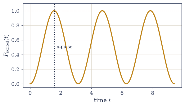
Fig. 523 Resonant Rabi oscillation. A two-level system driven exactly on resonance (\(\delta=0\), \(H=\tfrac{\Omega}{2}\sigma_x\)) and started in its lower level cycles completely between the two levels: the upper-level population is \(P_e(t)=\sin^2(\Omega t/2)\) (amber), reaching one at the \(\pi\)-pulse time \(\Omega t=\pi\) (marked), where the state is fully flipped. Driving the system for that exact duration is a quantum NOT gate; for half as long, a superposition. This is the elementary operation of magnetic resonance and of every gate-based qubit.

Exercise 6 — Off-resonant (generalized) Rabi oscillations

Repeat the driven two-level problem with a detuning \(\delta\ne0\), \(H=\tfrac{\delta} {2}\sigma_z+\tfrac{\Omega}{2}\sigma_x\). Show the oscillation becomes faster — at the generalized Rabi frequency \(\Omega_R=\sqrt{\Omega^2+\delta^2}\) — but shallower, reaching a maximum excited population \(\Omega^2/(\Omega^2+\delta^2)<1\) Eq. 530. Detuning reduces the transfer — resonance matters, and that selectivity is the basis of spectroscopy.

1. Build \(H=\tfrac{\delta}{2}\,\)SIGMA_Z\(+\tfrac{\Omega}{2}\,\)SIGMA_X for a few detunings \(\delta\).

2. Evolve from \(|0\rangle\) with your Exercise 1 evolve and compute \(P_e(t)\) as in Exercise 5.

3. Read off the maximum of \(P_e(t)\) (numpy.max) and confirm it equals \(\Omega^2/(\Omega^2+\delta^2)\).

4. Confirm the oscillation frequency is \(\Omega_R=\sqrt{\Omega^2+\delta^2}\) (e.g. the first return to \(P_e=0\) at \(t=2\pi/\Omega_R\)).

detuning δ:   max P_e (measured vs Ω²/(Ω²+δ²)):
  δ = 0.0:   1.0000  vs  1.0000     (Ω_R = √(Ω²+δ²) = 2.000)
  δ = 1.0:   0.8000  vs  0.8000     (Ω_R = √(Ω²+δ²) = 2.236)
  δ = 2.0:   0.5000  vs  0.5000     (Ω_R = √(Ω²+δ²) = 2.828)
  δ = 4.0:   0.2000  vs  0.2000     (Ω_R = √(Ω²+δ²) = 4.472)

Validation 6

✓  off-resonance the Rabi oscillation is faster (Ω_R=√(Ω²+δ²)) but shallower: the maximum excited population is Ω²/(Ω²+δ²) < 1   [max|Δ| = 6.87678e-06 (rtol=1e-06, atol=0.001)]

True

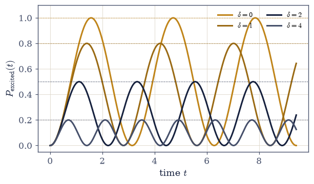
Fig. 524 Detuning kills the transfer. The upper-level population \(P_e(t)\) for a driven two-level system at several detunings \(\delta\) (resonant in amber, increasingly detuned in darker shades). As the drive moves off resonance the oscillation gets faster — its frequency is the generalized Rabi frequency \(\Omega_R=\sqrt{\Omega^2+\delta^2}\) — but shallower: the maximum reachable population drops to \(\Omega^2/(\Omega^2+\delta^2)\) (dotted lines), so a detuned drive can never fully flip the state. This selectivity — only a near-resonant drive transfers population — is what makes spectroscopy possible: the system responds to the frequency that matches its splitting.

Exercise 7 — Ehrenfest’s theorem and conservation laws (student)

Verify Ehrenfest’s theorem \(d\langle A\rangle/dt=i\langle[H,A]\rangle\) (\(\hbar=1\)) for a chosen observable, and use it to identify a conserved quantity — one that commutes with \(H\) Eq. 531. The commutator \([H,\cdot]\) is the quantum Poisson bracket (Volume II, canonical quantization), which is why commuting with \(H\) is what conservation means.

1. Take the precession Hamiltonian \(H=-\tfrac{\omega}{2}\sigma_z\) and the observable \(A=S_x\), with the state evolving from \(|{+}x\rangle\).

2. Compute \(d\langle A\rangle/dt\) by a centered finite difference of \(\langle S_x\rangle(t)\), evolving the state with the evolve you wrote in Exercise 1.

3. Compute \(i\langle[H,A]\rangle\) directly (the commutator via @, then numpy.vdot) at the same times.

4. Confirm the two agree.

5. Show that \(S_z\), which commutes with \(H\) (\([H,S_z]=0\)), is conserved — its expectation is constant.

d⟨Sx⟩/dt = -0.98545   vs   i⟨[H,Sx]⟩ = -0.98545   (agree: True)
[H, Sz] = 0: True;  ⟨Sz⟩(t) spread = 0.0e+00   (conserved)

Validation 7

✓  Ehrenfest's theorem: d⟨A⟩/dt = (i/ℏ)⟨[H,A]⟩; the rate of change of an expectation value is set by the commutator with H   [got -0.98545 vs expected -0.98545 (rtol=1e-06, atol=0.0001)]
✓  an observable that commutes with H is conserved: ⟨Sz⟩ is constant under precession about z

True

Exercise 8 — The state in motion, and why diagonalization is everything (synthesis)

The Hamiltonian generates a unitary flow \(U(t)=e^{-iHt/\hbar}\), and in its own eigenbasis that flow is nothing but a set of rotating phases \(e^{-iE_nt/\hbar}\). So the entire problem of dynamics collapses to one task — find the energy eigenstates — after which a stationary state stands still and a superposition beats at the Bohr frequencies. In the two-state system we watched this become a precessing spin and a driven oscillation, the very motions behind magnetic resonance, atomic clocks, and quantum gates. Ehrenfest’s theorem told us which quantities survive the motion (those commuting with \(H\)) and tied the commutator to the classical Poisson bracket.

There is no new computation here; the structure is the result. “Solve the Schrödinger equation” sounds like the hard part of quantum mechanics. It is the easy part — once you have the energy eigenstates, time is just phases. The hard part, the work of the rest of the volume, is finding them. The next notebook (§6.8) draws the geometry that makes all of this visible: the Bloch sphere, where a qubit’s state is a point, its evolution a rotation, and precession a literal spinning. Beyond the qubit, the same exponential will evolve wave packets and orbitals — the task is always the same, diagonalize \(H\).

Notebook summary

The dynamics postulate of §6.5, worked out — and the structure of all quantum motion.

• The time-evolution operator Eq. 527: \(U(t)=e^{-iHt/\hbar}\) solves \(i\hbar\dot U=HU\) and is unitary (probability conserved); scipy.linalg.expm and the spectral construction \(\sum_n e^{-iE_nt/\hbar}|n\rangle\langle n|\) agree.

• Stationary states Eq. 528: an energy eigenstate acquires only a phase, so its probabilities are frozen; a superposition beats at the Bohr frequencies \((E_n-E_m)/\hbar\). All dynamics is the interference of energy phases — so diagonalizing \(H\) solves the motion.

• Larmor precession Eq. 529: \(\langle S_x\rangle=\tfrac12\cos\omega t\), \(\langle S_y\rangle =-\tfrac12\sin\omega t\), \(\langle S_z\rangle\) conserved — a classical precession from unitary evolution (NMR).

• Rabi oscillations Eq. 530: on resonance \(P_e=\sin^2(\Omega t/2)\) (complete cycling, the \(\pi\)-pulse gate); off resonance faster (\(\Omega_R=\sqrt{\Omega^2+\delta^2}\)) but shallower (\(P_e^{\max}=\Omega^2/(\Omega^2+\delta^2)\)).

• Ehrenfest’s theorem Eq. 531: \(d\langle A\rangle/dt=(i/\hbar)\langle[H,A]\rangle\); observables commuting with \(H\) are conserved, and \([H,\cdot]\) is the quantum Poisson bracket.

Solving the Schrödinger equation is the easy part — once the energy eigenstates are in hand, time is just phases. Finding them is the rest of the volume.

Outlook

• The Bloch sphere (§6.8): qubit states as points, unitary evolution as rotation, precession made geometric.

• Continuous-system dynamics (§6.10–§6.13): evolving wave packets, the time-dependent Schrödinger equation by split-step and Crank–Nicolson.

• Driven transitions and Fermi’s golden rule (§6.24): Rabi physics in the many-level setting, time-dependent perturbation theory.

• The classical limit: the commutator as the Poisson bracket (Volume II), Ehrenfest \(\to\) Newton — canonical quantization \(\{\cdot,\cdot\}\to\tfrac{1}{i\hbar}[\cdot,\cdot]\).

• Cross-reference §6.2 (the exponential map), §6.3 (functions of operators), §6.5 (the dynamics postulate), §6.6 (commutators, conservation), Volume II (Poisson brackets), and forward to §6.8, §6.10–§6.13, §6.24.

Take this notebook with you

Use the download button (↓) in the toolbar above to save this notebook and run it yourself. The published notebooks ship without worked solutions; if you would like the reference solutions — to teach from or to check your own work — get in touch: hello@ramador.me.