


6.13 Scattering, Tunneling, and Wave-Packet Dynamics#
Notebook overview#
Every notebook of Movement II so far has found stationary states — the bound levels of a well, the rungs of the oscillator, things that sit still. This one, the movement’s finale, finally introduces motion. A particle that is not bound is a wave packet — a normalizable superposition of the non-normalizable momentum eigenstates of §6.9 — and watching it move shows everything the classical picture forbids. It spreads as it travels (unlike the oscillator’s coherent state, which a restoring force holds together); it reflects off barriers it has more than enough energy to cross; and it tunnels through barriers it could never surmount classically. That last effect alone explains how stars burn, how nuclei decay, and how we image single atoms.
The engine is a small, beautiful algorithm: the split-step Fourier propagator. The time-evolution operator \(e^{-iHt/\hbar}\) of §6.7 does not factor simply, because the kinetic and potential pieces of \(H=\hat T+\hat V\) do not commute — but the Strang splitting \(e^{-iH\,dt/\hbar}\approx e^{-i\hat V dt/2\hbar}e^{-i\hat T dt/\hbar}e^{-i\hat V dt/2\hbar}\) is accurate to \(O(dt^3)\) per step, and it works because \(\hat V\) is diagonal in position (a multiplication) while \(\hat T=\hat p^2/2m\) is diagonal in momentum (a multiplication after a Fourier transform). So each step is a phase, an FFT, a phase, an inverse FFT, a phase — every factor a pure phase, so the propagator is unitary by construction and conserves probability exactly. We derive it, verify its unitarity to a part in \(10^{12}\), and turn it loose.
Then the physics. A free packet spreads — we derive the spreading law in-cell rather than quote it, minding the subtle difference between the wave-function width and the probability-density width. Sent at a barrier it splits into transmitted and reflected parts with \(T+R=1\). When the barrier is higher than the particle’s energy, classical mechanics forbids transmission entirely, yet the packet tunnels through with a probability that falls exponentially with the barrier width — the mechanism of alpha decay, the scanning tunneling microscope, and the tunnel diode. And when the energy exceeds the barrier, classical mechanics predicts certain transmission, yet the packet partly reflects — except at resonances, where standing-wave interference inside the barrier makes it perfectly transparent (the Ramsauer–Townsend effect, the same physics as an anti-reflection coating).
As in every Volume VI notebook, each exercise opens with a crystal-clear statement and enumerated parts, each naming the exact operation — the split-step propagator via numpy.fft.fft/ifft/
fftfreq, and numpy.trapezoid (or masked sums) for the transmission and reflection probabilities.
Conventions and method notes. \(\hbar=m=1\). The grid is \(N\) points on a box \([-L/2,L/2]\) with the periodic boundaries of the FFT, so the box must be large enough that the packet never wraps around within the simulation (we use \(L=160\), comfortably larger than the packet’s travel; absorbing boundaries are the alternative for long runs). A Gaussian packet is \(\psi\propto e^{-(x-x_0)^2/2\sigma^2} e^{ik_0x}\) — note that with this wave-function width \(\sigma\), the probability-density width (standard deviation of \(|\psi|^2\)) is \(\sigma/\sqrt2\), a distinction we keep careful track of. See Griffiths (scattering, tunneling); Tannor, A Time-Dependent Perspective (the split-step method); and Notebooks §6.7 (the time-evolution operator), §6.9 (momentum eigenstates, the Fourier transform), §6.11 (the leaking tails, double-well tunneling), §6.12 (the non-spreading coherent state).
Theory in brief#
Wave packets and free motion#
A physical travelling particle is a normalizable wave packet, a superposition of momentum eigenstates (§6.9),
A free packet spreads: its different-\(k\) components move at different speeds, so it broadens over time — the contrast to the coherent state of §6.12, which a restoring potential prevents from spreading. We derive the density-width spreading law in-cell.
The split-step Fourier propagator#
To evolve \(\psi\) under \(H=\hat T+\hat V\), use the Strang splitting
exploiting that \(\hat V\) is diagonal in position and \(\hat T=\hat p^2/2m\) is diagonal in momentum. Each step: multiply by \(e^{-iV dt/2\hbar}\) (position), FFT, multiply by \(e^{-i\hbar k^2 dt/2m}\) (momentum), inverse FFT, multiply by \(e^{-iV dt/2\hbar}\). Every factor is a pure phase, so the propagator is unitary — probability is conserved exactly.
Barrier scattering: transmission and reflection#
A packet of mean energy \(E\) sent at a rectangular barrier (height \(V_0\), width \(a\)) splits,
into a transmitted part (probability \(T\), beyond the barrier) and a reflected part (\(R\)). The packet has an energy spread, so its \(T,R\) match the plane-wave formulas approximately.
Tunneling#
When \(V_0>E\) the barrier is classically forbidden, yet the quantum packet tunnels with nonzero \(T\) that falls exponentially with the width,
the mechanism of alpha decay, the scanning tunneling microscope (its exponential distance-sensitivity gives atomic resolution), the tunnel diode, and stellar fusion. The wave function does not vanish in the barrier — it decays exponentially (the leaking tails of §6.11, now traversed).
Over-barrier reflection and resonances#
When \(E>V_0\), classical mechanics predicts certain transmission, yet the packet partly reflects (\(R>0\)) — except at resonances,
where the barrier width is a whole number of interior half-wavelengths and standing-wave interference makes it transparent (the Ramsauer–Townsend effect; an anti-reflection coating).
Setup#
The data are the series palette, the conventions \(\hbar=m=1\), the simulation grid (\(N=2048\) points
on a box of length \(L=160\), wide enough that a packet never wraps around the periodic FFT
boundaries), and two given formulas. gaussian_packet is the specimen every run is launched with —
the packet of Eq. 561, written with a wave-function width \(\sigma\) and normalized by
numpy.trapezoid. plane_wave_T is the textbook closed form for a plane wave crossing a
rectangular barrier; it is here only as the analytic yardstick the simulated probabilities are held
against, never as the thing being computed. The one instrument is density_width, a pair of moment
integrals that reads the standard deviation of \(|\psi|^2\) off the grid. The two methods this
notebook is named for are not here: you write the split-step propagator in Exercise 1 and the
transmitted and reflected probabilities in Exercise 3, and every exercise after them runs on the
ones you wrote.
The Setup below holds this notebook’s data and instruments — nothing you are asked to build. It is collapsed so the building stays yours; expand it whenever you want the details.
Exercise 1 — The split-step Fourier propagator#
The engine of everything that follows is the Strang splitting \(e^{-iH\,dt/\hbar}\approx e^{-i
\hat V dt/2\hbar}e^{-i\hat T dt/\hbar}e^{-i\hat V dt/2\hbar}\), accurate to \(O(dt^3)\) per step
Eq. 562. It works because each piece of \(H\) is a mere multiplication in the right
representation: \(\hat V\) is diagonal in position (multiply by \(e^{-iVdt/2\hbar}\)) and \(\hat T=\hat
p^2/2m\) is diagonal in momentum (multiply by \(e^{-i\hbar k^2dt/2m}\) after numpy.fft.fft, with
\(k=2\pi\,\)numpy.fft.fftfreq). One step is therefore half-\(V\) \(\to\) FFT \(\to\) full-\(T\) \(\to\) IFFT
\(\to\) half-\(V\), and since every one of those factors is a pure phase, the propagator is unitary
by construction — no discretization can leak probability, and the norm \(\int|\psi|^2dx\) is
conserved to machine precision however long the run. This is the workhorse of time-dependent
quantum dynamics, and it is the propagator the rest of the notebook is built on.
Write
split_step(psi, V, dt, n_steps, x), returning the wave function advanced byn_stepsStrang steps of sizedton the gridxunder the static potentialV. Write this one yourself — the implementation is the lesson.Evolve a free packet (\(V=0\)) for many steps and check the norm \(\int|\psi|^2dx\) against its initial value (
numpy.trapezoid), confirming the drift is at the level of round-off.
norm at t=0: 1.0000000000
norm after 2000 split-step iterations: 1.0000000000
drift: 2.0e-13  (unitary by construction — every factor is a pure phase)
Validation 1#
✓ the split-step Fourier propagator is unitary — probability is conserved over thousands of steps [got 1 vs expected 1 (rtol=1e-05, atol=1e-09)]
True
Exercise 2 — Free-packet spreading#
A free packet does not keep its shape. Unlike the coherent state of §6.12, which a restoring force holds rigidly together, a packet with no potential acting on it spreads: it is a superposition of momentum components, and the faster ones outrun the slower. The wave-function-vs-density distinction matters throughout — a Gaussian of wave-function width \(\sigma\) has \(|\psi|^2\propto e^{-x^2/\sigma^2}\), whose standard deviation is \(\sigma/\sqrt2\), so the density width starts at \(\sigma/\sqrt2\) and not at \(\sigma\) Eq. 561. The law it then follows is worth deriving rather than quoting: the momentum amplitude is \(\varphi(k)\propto e^{-\sigma^2k^2/2}\) (Fourier reciprocity, §6.9), free evolution attaches \(e^{-i\hbar k^2t/2m}\) to each component, and carrying that through gives \(w(t)=(\sigma/\sqrt2)\sqrt{1+(\hbar t/m\sigma^2)^2}\).
Build a stationary Gaussian (\(k_0=0\)) of wave-function width \(\sigma\) and confirm its density width at \(t=0\) is \(\sigma/\sqrt2\) (the Setup’s
density_widthinstrument).Evolve it freely with the
split_stepyou wrote in Exercise 1 and measure the density width at several times.Confirm the simulated widths grow monotonically and match the derived law \(w(t)\) above.
wave-function width σ = 3.0; density width at t=0 = 2.1213 (= σ/√2 = 2.1213)
times:            [ 0.  5. 10. 20. 40.]
simulated width:  [2.121 2.427 3.171 5.169 9.664]
derived law w(t): [2.121 2.427 3.171 5.169 9.664]   (monotonic and matching)
Validation 2#
✓ a free wave packet spreads: the density width grows monotonically and matches the in-cell-derived law w(t)=(σ/√2)√(1+(ℏt/mσ²)²)
True
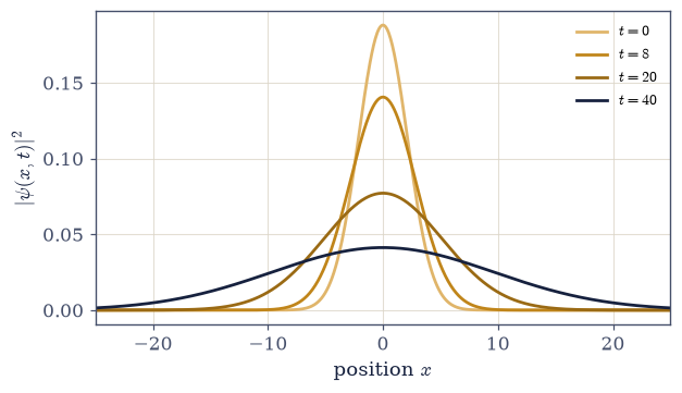
Fig. 544 A free packet spreads. The probability density \(|\psi(x,t)|^2\) of a free Gaussian packet at successive times (light to dark): it stays Gaussian but broadens and flattens, its width growing as \(w(t)=(\sigma/\sqrt2)\sqrt{1+(\hbar t/m\sigma^2)^2}\) — derived in-cell from the momentum distribution, not quoted. The cause is dispersion: the packet is a superposition of momentum components (§6.9), and the faster ones outrun the slower, smearing the packet out. This is the sharp contrast to the harmonic oscillator’s coherent state (§6.12), which a restoring force holds rigidly together. A free quantum particle does not stay localized — it disperses, the more quickly the more sharply it began.#
Exercise 3 — Barrier scattering: \(T+R=1\)#
A packet sent at a barrier does not choose: it splits, one part carrying on past the barrier and one part coming back. Probability splits with it, and because the propagator is unitary none of it is lost, so the two pieces must add to one, \(T+R=1\) Eq. 563. Turning that statement into numbers takes an operational definition of \(T\) and \(R\): once the collision is over and the two pieces have separated, \(T\) is the probability still to the right of the barrier and \(R\) the probability back to its left, each the integral of \(|\psi|^2\) over that region. Only the timing and the bookkeeping need care — the packet must have fully scattered before the reading is taken, and the two integration regions must be kept a little clear of the barrier so that density still sitting inside it is counted in neither.
Write
transmission_reflection(psi, x, barrier_half_width, pad=5.0), returning \((T,R)\) as thenumpy.trapezoidintegrals of \(|\psi|^2\) over \(x>a/2+\)padand \(x<-a/2-\)pad.Build a rectangular barrier (height \(V_0\), width \(a\)) and a packet of mean momentum \(k_0\), hence mean energy \(E=\hbar^2k_0^2/2m\).
Evolve with the
split_stepyou wrote in Exercise 1 until the packet has fully scattered (the transmitted and reflected parts are clear of the barrier), then read off \(T\) and \(R\).Confirm \(T+R=1\) to high precision — probability splits, and is conserved.
packet mean energy E = 2.000, barrier V0 = 1.5 (E > V0, classically certain transmission)
T = 0.7256,  R = 0.2743,  T + R = 1.0000
  (R > 0 even though E > V0 — a purely quantum reflection, explored in Exercise 6)
Validation 3#
✓ scattering conserves probability: T + R = 1 (the split-step propagator is unitary) [got 0.999985 vs expected 1 (rtol=0.002, atol=1e-09)]
True
Exercise 4 — Tunneling through a forbidden barrier#
Raise the barrier above the packet’s energy, \(V_0>E\), and classical mechanics is unambiguous: the
particle cannot be there, so it cannot get across. The wave function disagrees. Inside the
forbidden region it does not vanish but decays exponentially, \(\psi\sim e^{-\kappa x}\) with
\(\kappa=\sqrt{2m(V_0-E)}/\hbar\) — the leaking tails of §6.11, now
traversed rather than merely peeked into — and if the barrier is thin enough, enough amplitude
survives to the far side to re-emerge as a travelling packet with nonzero \(T\) Eq. 564.
This is tunneling, a quantum effect with no classical analogue whatsoever. The plane-wave
plane_wave_T of the Setup gives the analytic value to compare against; the agreement is only
approximate, because a packet carries a spread of energies rather than the single \(E\) the
closed form assumes.
Set \(V_0>E\) (the barrier is classically impenetrable) and evolve the packet into it with the
split_stepyou wrote in Exercise 1.Measure \(T\) and \(R\) with your Exercise 3
transmission_reflection.Confirm \(T>0\) — the packet tunnels — with \(T+R=1\) still holding, and compare \(T\) to
plane_wave_Tat the packet’s mean energy.
V0 = 4.0 > E = 2.00 (classically forbidden), κ = 2.000
tunneling: T = 0.0944 > 0,  R = 0.9055,  T + R = 0.9999
  analytic plane-wave T = 0.0707  (approximate: the packet has an energy spread)
Validation 4#
✓ a packet tunnels through a classically forbidden barrier (T>0 for V0>E), with T+R=1 and T near the analytic plane-wave value
True
Fig. 545 Tunnelling through a wall, animated. A wave packet (amber) approaches a barrier higher than its energy (grey) — a wall a classical particle could never cross. Most of it reflects, as classical intuition expects, but a small part tunnels straight through and emerges on the far side, because the wave function does not vanish inside the forbidden region: it decays exponentially, and if the barrier is thin enough, enough survives to the other side to re-emerge as a travelling packet. The transmitted fraction is tiny and exponentially sensitive to the barrier’s width — which is exactly why this effect, invisible in daily life, runs the alpha decay of nuclei, the scanning tunnelling microscope’s atomic resolution, and the tunnel diode. The wall is real; the particle is real; and there it is on the other side.#
Exercise 5 — Exponential suppression of tunneling#
Tunneling happens, but it is exquisitely sensitive to how far the particle has to tunnel. For a thick barrier the amplitude decays as \(e^{-\kappa a}\) across it and the probability as the square, so the transmission falls exponentially with the width: \(\ln T\) is linear in \(a\) with slope \(-2\kappa\), \(\kappa=\sqrt{2m(V_0-E)}/\hbar\) Eq. 564. That steepness is the reason a small change in a barrier — a slightly larger nucleus, a slightly wider vacuum gap — changes a tunneling rate or a tunneling current by orders of magnitude, which is what spreads alpha-decay half-lives over some twenty decades and what gives the scanning tunneling microscope its resolution (Exercise 7).
Compute the analytic tunneling probability \(T\) (the Setup’s
plane_wave_T) for a series of barrier widths \(a\).Fit \(\ln T\) against \(a\) in the thick-barrier regime with
numpy.polyfitand confirm the slope is \(-2\kappa\).Plot \(T\) against \(a\) on a logarithmic scale, where the exponential law is a straight line.
κ = 2.000,  so the expected slope −2κ = -4.000
fitted slope of ln T vs a (thick-barrier regime): -3.998
  → T falls by a factor of 55 per unit of barrier width
Validation 5#
✓ tunneling is exponentially suppressed with barrier width: ln T is linear in a with slope −2κ [got -3.99824 vs expected -4 (rtol=0.05, atol=1e-09)]
True
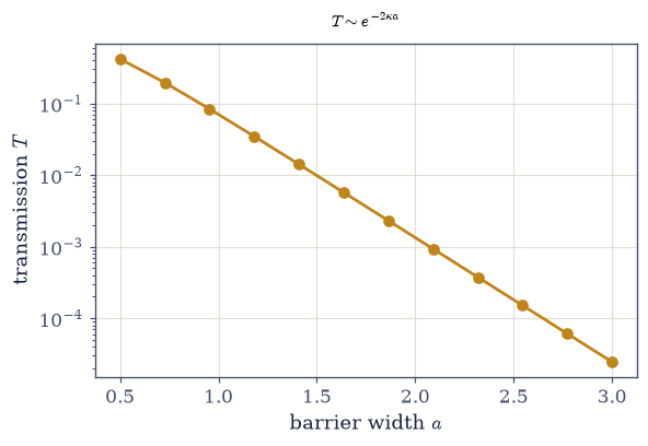
Fig. 546 Tunnelling is exponentially sensitive to the barrier. The transmission probability \(T\) through a forbidden barrier against its width \(a\), on a log scale (amber): a straight line of slope \(-2\kappa\), so \(T\sim e^{-2\kappa a}\). Widening the barrier by one unit drops the transmission by a large factor; a barrier twice as thick is not twice as opaque but exponentially more so. This steepness is the whole reason tunnelling, though always present, is invisible at macroscopic scales — and it is also what makes the scanning tunnelling microscope work: because the tunnelling current changes about tenfold for every ångström of tip–surface gap, the instrument can resolve single atoms from the current alone (Exercise 7).#
Exercise 6 — Over-barrier reflection and resonant transmission#
Tunneling is the famous surprise, but the opposite case is just as strange. When the packet has more than enough energy to clear the barrier, \(E>V_0\), classical mechanics predicts certain transmission — and yet part of it comes back. The reflection is a purely quantum response to the abrupt edges of the potential, exactly as light partly reflects off a change of refractive index however transparent the glass. The exception is a set of special energies: when the interior wavenumber \(k_{\text{in}}=\sqrt{2m(E-V_0)}/\hbar\) fits a whole number of half-wavelengths across the barrier, \(k_{\text{in}}a=n\pi\), the reflections off the two edges interfere destructively and the barrier becomes perfectly transparent, \(T=1\) Eq. 565. These are resonances — the Ramsauer–Townsend effect, which makes noble gases nearly invisible to slow electrons, and the same standing-wave physics as an anti-reflection coating on a lens.
For \(E>V_0\), compute the analytic transmission \(T(E)\) (the Setup’s
plane_wave_T) across a range of energies at fixed barrier height and width.At a representative non-resonant energy, confirm \(T<1\) — so \(R=1-T>0\), a reflection classical mechanics forbids.
Compute the resonance energies from \(k_{\text{in}}a=n\pi\), i.e. \(E_n=V_0+(n\pi/a)^2\hbar^2/2m\), and confirm \(T=1\) at each of them.
E > V0 = 2.0:  at E = 2.50, T = 0.7773  (R = 0.2227 > 0, classically forbidden reflection)
resonance energies (k_in·a = nπ): [ 2.79   5.158  9.106 14.633 21.739]
transmission at resonances:        [1. 1. 1. 1. 1.]  (= 1: perfect transmission, Ramsauer–Townsend)
Validation 6#
✓ over-barrier reflection occurs (R>0 for E>V0) except at resonances k_in·a=nπ, where transmission is perfect (T=1)
True
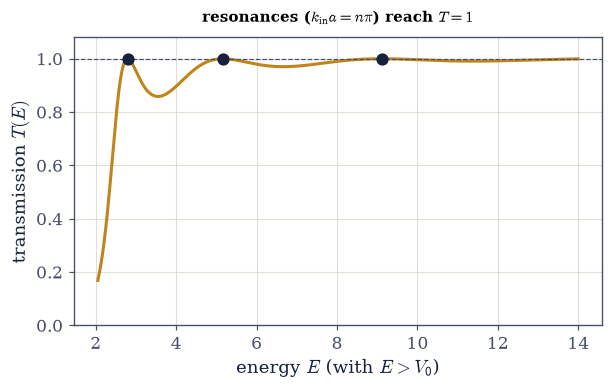
Fig. 547 Over-barrier reflection and transmission resonances. The transmission probability \(T(E)\) for a packet whose energy exceeds the barrier height \(V_0\) (amber). Classically the particle would always cross (\(T=1\)), but quantum mechanically \(T\) dips below one between the peaks — the packet partly reflects off a barrier it has the energy to clear, a purely quantum effect of the sharp potential edges. At special energies, though, \(T\) returns exactly to one (dots): these are resonances, where the barrier width is a whole number of interior half-wavelengths (\(k_{\text{in}}a=n\pi\)) and the reflections off the two edges interfere destructively, making the barrier perfectly transparent. This is the Ramsauer–Townsend effect — noble gases are nearly transparent to slow electrons — and it is the same standing-wave physics as an anti-reflection coating on a lens.#
Exercise 7 — Tunneling and the scanning tunneling microscope (student)#
The tunneling of this notebook is not only a curiosity of model potentials: it is the working principle of a real instrument. In a scanning tunneling microscope the vacuum gap between a sharp metal tip and a surface is a barrier of height the work function \(W\approx4.5\,\)eV, and electrons cross it by tunneling. The decay constant in laboratory units is \(\kappa=\sqrt{2m_eW}/\hbar\approx0.51\sqrt{W/\mathrm{eV}}\ \text{Å}^{-1}\), and the current scales as the transmission, \(I\propto e^{-2\kappa d}\) with the gap \(d\) Eq. 564.
Compute \(\kappa\) for \(W\approx4.5\,\)eV, in inverse ångströms.
Compute the ratio of currents for gaps differing by \(1\,\)Å and show it is roughly an order of magnitude.
Say what that buys the instrument: because the current changes about tenfold per ångström, a sub-ångström height change is easily read off the current — so the STM maps a surface atom by atom.
work function W = 4.5 eV → κ = 1.086 Å⁻¹
current ratio for a 1 Å change in gap: I(d)/I(d+1Å) = e^(2κ·1Å) = 8.8×
  → roughly an order of magnitude per ångström: a tiny height change is a large, readable current change
This exponential distance-sensitivity is what gives the STM its atomic resolution.
Validation 7#
✓ the STM's atomic resolution comes from the exponential distance-dependence of tunneling: the current changes ~an order of magnitude per ångström of gap
True
Exercise 8 — Quantum motion: spreading, tunneling, and the failure of the classical picture (synthesis)#
A particle that is not bound is a wave packet, and watching it move — by splitting the evolution operator into a position kick and a momentum drift, a phase and a Fourier transform and a phase — shows everything the classical picture forbids. It spreads as it travels, because it is a superposition of momenta that disperse. It reflects off barriers it has the energy to cross, because of the sharp edges. And it tunnels through barriers it could never surmount, because the wave function is never quite zero in the forbidden region. Tunnelling alone explains how stars burn, how nuclei decay, and how we image single atoms.
There is no new computation to do here; the catalogue of quantum motions is itself the result. The split-step method is almost embarrassingly simple — a phase, a Fourier transform, a phase — yet it shows a particle tunnelling through a wall in real time. With this, Movement II is complete: we took the formalism to the continuum (§6.9), solved the bound states by diagonalization (§6.10, §6.11), met the universal oscillator three ways (§6.12), and set wave packets moving through barriers (§6.13) — the two systems, the oscillator and the barrier, that physics returns to most. Movement III now adds the dimension we have been missing: angular momentum, built from the very same ladder algebra of §6.12, assembles the spherical world and, at its summit, the hydrogen atom.
Notebook summary#
Quantum motion through the continuous spectrum — the close of Movement II.
Wave packets Eq. 561: a free particle is a normalizable superposition of momentum eigenstates (§6.9), with group velocity \(\hbar k_0/m\); its density width is \(\sigma/\sqrt2\).
The split-step propagator Eq. 562: the Strang splitting (
numpy.fft.fft/ifft), half-\(V\)/full-\(T\)/half-\(V\) — unitary by construction, norm conserved to \(\sim10^{-12}\).Spreading Eq. 561: a free packet broadens as \(w(t)=(\sigma/\sqrt2)\sqrt{1+(\hbar t/m \sigma^2)^2}\) (derived in-cell) — unlike the coherent state (§6.12).
Scattering and tunnelling Eq. 563, Eq. 564: \(T+R=1\); for \(V_0>E\) the packet tunnels with \(T\sim e^{-2\kappa a}\) — alpha decay, the STM, the tunnel diode.
Over-barrier resonances Eq. 565: for \(E>V_0\), \(R>0\) except at \(k_{\text{in}}a=n\pi\) where \(T=1\) (Ramsauer–Townsend, an anti-reflection coating).
A phase, a Fourier transform, a phase — and a particle tunnels through a wall in real time. Movement II is complete; Movement III adds the missing dimension.
Outlook#
Three-dimensional scattering: cross sections, partial waves, the Born approximation (a horizon; time-dependent transitions are §6.24).
The angular-momentum algebra and three dimensions (Movement III, §6.14): the same ladder method of §6.12, now for rotations — building toward the hydrogen atom.
Tunnelling in the wild: alpha decay (Gamow), the STM, Josephson junctions, stellar fusion (horizons; the STM ties to surface science).
Absorbing boundary conditions for larger time-dependent simulations (a computational horizon).
Cross-reference §6.7 (time evolution), §6.9 (momentum eigenstates, the Fourier transform), §6.11 (leaking tails, double-well tunnelling), §6.12 (the non-spreading coherent state), and forward to §6.14, §6.24.