1.2 The Damped, Driven Pendulum

1.2 The Damped, Driven Pendulum#

    Elementary Computational Physics
  

Volume I — Elementary Mechanics Notebook 1.2

From a linear resonance curve to the period-doubling road to chaos — one nonlinear oscillator, three regimes.

Level · intermediate • Est. · 60–90 min

    Raymond Amador
    v1.4.0  ·  2026-07-31  · 
          CC BY 4.0 (text) / MIT (code)
  

Notebook overview#

The pendulum is the first oscillator every student meets, and in the small-angle limit it is utterly tame: a single sine wave. Add damping and a periodic push, then let the swing grow large enough that $\sin\theta$ can no longer be replaced by $\theta$, and the same one-degree-of-freedom system becomes one of the cleanest textbook routes to chaos. It is the simplest place to watch a period-doubling cascade unfold.

We will (1) implement the equations of motion, (2) recover the simple-harmonic period in the small-angle limit, (3) measure the damped decay rate and shifted frequency, (4) reproduce the linear resonance curve from a driven steady state, (5) locate the resonance peak, (6) build a bifurcation diagram showing the period-doubling cascade, (7) confirm chaos at the canonical parameters by measuring a positive Lyapunov exponent, and (8) animate the damped free decay. Two animations punctuate the notebook: a worked one (the chaotic bob swinging on its attractor) in Exercise 7, and one you build in Exercise 8.

How to read the checks. Each exercise ends with a validation that compares our result to an expected physical fact. A ✗ does not by itself mean the answer is wrong: it means the output didn’t match what the check expected, which may be a real error, a different-but-valid convention (a sign, a unit, an array order), or simply too tight a tolerance. Treat a ✗ as a prompt to locate the discrepancy; passing is strong evidence of correctness, not proof.

Scope. This is a working review, not a textbook chapter. For the mechanics of the pendulum see Nolting, Theoretical Physics 1 [Nol16]; for the bifurcation and chaos picture, Strogatz, Nonlinear Dynamics and Chaos [Str15].

Theory in brief#

Equation of motion and nondimensionalisation#

A pendulum of mass $m$ on a rod of length $\ell$, with a linear (viscous) damping torque $-b\dot\theta$ and a sinusoidal drive torque $\tau_0\cos(\Omega t)$, obeys the torque balance

\[ m\ell^2 \ddot\theta = -b\,\dot\theta - m g \ell \sin\theta + \tau_0 \cos(\Omega t). \]

Divide by $m\ell^2$ and introduce the natural frequency $\omega_0 = \sqrt{g/\ell}$. Measuring time in units of $1/\omega_0$ (so the dimensionless time is $\omega_0 t$, and frequencies are measured in units of $\omega_0$) collapses every system onto the Baker–Gollub form

(103)#\[\ddot\theta + \frac{1}{q}\,\dot\theta + \sin\theta = A\cos(\omega_d t)\]

with just three numbers: the quality factor $q$ (the damping rate is $1/q$), the dimensionless drive amplitude $A$, and the drive frequency $\omega_d = \Omega/\omega_0$. We carry the state $\mathbf s = (\theta, \omega)$ with $\omega \equiv \dot\theta$, so the second-order ODE becomes the first-order system $\dot\theta = \omega$, $\dot\omega = -\omega/q - \sin\theta + A\cos(\omega_d t)$.

Small-angle linear limit#

For $|\theta|\ll 1$, $\sin\theta \approx \theta$ and Eq. 103 becomes the damped, driven linear oscillator

(104)#\[\ddot\theta + \tfrac1q\dot\theta + \theta = A\cos(\omega_d t),\]

which we can solve exactly, giving us three independent checks on the integrator (Taylor, Classical Mechanics, Ch. 5, carries the solution of the damped, driven linear oscillator out in full; we quote its three results).

Free, undamped ($A=0$, $q\to\infty$): Eq. 104 is simple harmonic motion at $\omega_0 = 1$, i.e. period $2\pi$.

Free, underdamped ($A=0$): the amplitude decays under the envelope $e^{-t/(2q)}$ while oscillating at the shifted frequency

(105)#\[\omega_1 = \sqrt{1 - \tfrac{1}{4q^2}}.\]

Driven steady state: after transients die, the response is sinusoidal at the drive frequency with amplitude

(106)#\[\Theta(\omega_d) = \frac{A}{\sqrt{(1-\omega_d^2)^2 + (\omega_d/q)^2}},\]

a resonance curve that peaks at

(107)#\[\omega_d^\star = \sqrt{1 - \tfrac{1}{2q^2}}.\]

The nonlinear regime#

Once $A$ is large enough to drive the pendulum to wide swings, the $\sin\theta$ nonlinearity matters and the tidy linear picture fails. Holding $q$ and $\omega_d$ fixed and turning $A$ up, the steady response loses stability in a period-doubling cascade: a period-1 orbit (closing after one drive period) gives way to period-2, then period-4, 8, …, accumulating at a critical drive beyond which the motion is chaotic: bounded, deterministic, yet sensitive to initial conditions. The canonical chaotic parameters used throughout the literature are $$ q = 2, \qquad A = 1.5, \qquad \omega_d = \tfrac{2}{3}. $$

The physical setup#

A bob of mass $m$ hangs from a pivot on a rigid rod of length $\ell$, swinging to an angle $\theta$ from the downward vertical. Two extra torques act on top of gravity: a viscous damping $-b\dot\theta$ that opposes the motion, and an external sinusoidal drive $\tau_0\cos(\Omega t)$. Those three ingredients (restoring gravity, damping, periodic forcing) are the whole of Eq. 103.

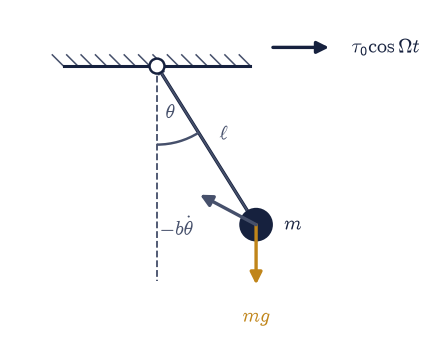
../../_images/11ee08c9b786b90c1df38ef47715fd2ad64ee15046bec57b38f7d797a5d8234c.png — Fig. 84 The damped, driven pendulum: a bob of mass $m$ on a rigid rod of length $\ell$ swings to angle $\theta$ from the downward vertical (dashed) under gravity $mg$, a viscous damping torque $-b\dot\theta$ opposing the motion, and an external sinusoidal drive $\tau_0\cos\Omega t$ of amplitude $\tau_0$ and angular frequency $\Omega$.#

Setup#

Data only: the imports, a seeded generator, and the canonical chaotic parameters $q=2$, $A=1.5$, $\omega_d=2/3$ that Exercises 6 and 7 share. Every piece of machinery this notebook is about — the equation of motion Eq. 103, the integration wrapper, the crossing- and peak-finders that measure period and decay, the steady-state amplitude behind the resonance curve, and the stroboscopic Poincaré sampler that exposes the cascade — you build in the exercise where it is earned.

The Setup below holds this notebook’s data and instruments — nothing you are asked to build. It is collapsed so the building stays yours; expand it whenever you want the details.

Exercise 1 — Implement the equations of motion#

Everything in this notebook runs on the one second-order equation Eq. 103. A solver needs it as a first-order system, so we carry the state $\mathbf s = (\theta, \omega)$ with $\omega \equiv \dot\theta$, and carrying $q$, $A$, $\omega_d$ as arguments lets every later exercise select its regime by passing different numbers. In the small-angle limit the restoring term is linear, so an undriven, undamped displacement $\theta$ must feel the acceleration $-\omega_0^2\theta = -\theta$ (recall $\omega_0 = 1$) — the fact the check below leans on.

Write the right-hand side rhs(t, s, q, A, wd) returning $(\dot\theta, \dot\omega)$ for Eq. 103: unpack $\mathbf s = (\theta, \omega)$, whose first derivative is just $\dot\theta = \omega$, then return $\dot\omega = -\omega/q - \sin\theta + A\cos(\omega_d t)$, reading the three terms straight off Eq. 103. Write this one yourself — the implementation is the lesson.
Certify it in the small-angle limit: with drive and damping switched off, evaluate the angular acceleration at $\theta = 10^{-3}$ and confirm it is $-\theta$.

Validation 1 — the small-angle restoring force#

The check reads the angular acceleration returned by rhs at $\theta = 10^{-3}$ with the drive and damping switched off, and compares it to the linear restoring acceleration $-\omega_0^2\theta = -\theta$.

✓  small-angle restoring force is -ω₀²θ   [got -0.001 vs expected -0.001 (rtol=1e-06, atol=1e-09)]

True

Exercise 2 — Small-angle free oscillation recovers the SHM period#

The first check on the integrator is the tamest limit of Eq. 104: with no drive and negligible damping, a small swing is simple harmonic motion at $\omega_0 = 1$, period $2\pi$. If the code can’t reproduce that, nothing downstream is trustworthy.

Write integrate(s0, t_end, q, A, wd, ...), a wrapper that runs your Exercise 1 rhs through scipy.integrate.solve_ivp (DOP853, rtol=1e-10, atol=1e-12) on a dense uniform t_eval and hands back the solution; every later exercise integrates through it. Use it on the undriven ($A=0$), essentially undamped ($q$ enormous) pendulum from a small angle.
Write zero_crossing_times(t, x), which linearly interpolates the times at which a sampled signal changes sign; measure the period from successive zero crossings of $\theta(t)$ and confirm it equals $2\pi/\omega_0 = 2\pi$. (Note the densely sampled t_eval: a sparse adaptive solution drawn with straight segments looks jagged even when the numbers are right.)

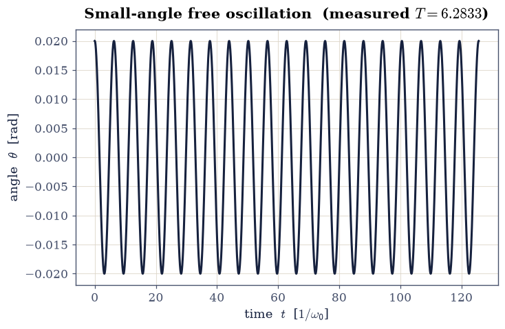
../../_images/84dac225084dc51ceee1b0cb0febcc61fdafe997ddbb00aa39bbb3f656355382.png

✓  small-angle period is 2π/ω₀   [got 6.28334 vs expected 6.28319 (rtol=0.002, atol=1e-09)]

True

Exercise 3 — Damped free decay: rate and frequency#

Turn damping on (still no drive) and Eq. 104 predicts two things at once: the amplitude decays under the envelope $e^{-t/(2q)}$, and the oscillation frequency drops to $\omega_1$ from Eq. 105. Both are measurable from a single free-decay run.

Set $q=5$, $A=0$ and integrate from a small angle on a dense t_eval with the integrate wrapper you wrote in Exercise 2.
Measure the decay rate from the upper envelope of the peaks (write refined_maxima, which locates the peaks with sub-sample parabolic refinement, then numpy.polyfit on the log) and compare it to $1/(2q)$.
Measure the frequency from the zero crossings (your Exercise 2 zero_crossing_times) and compare it to $\omega_1$ of Eq. 105. Overlay the analytic envelope on $\theta(t)$.

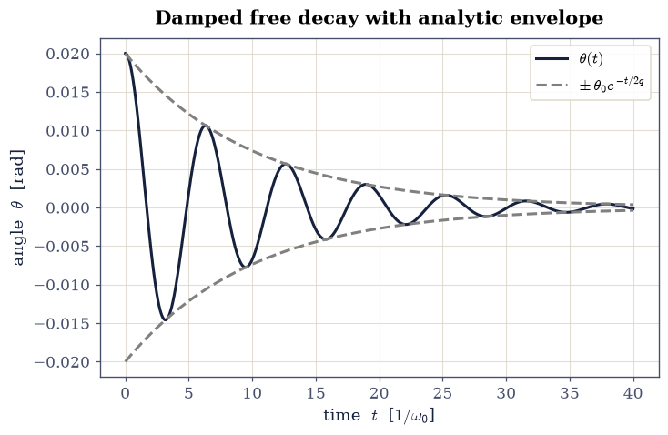
../../_images/2f7804f9987cc795f46ab04d8f4d717ee33bfdcdd80169102ebbc27356e737b8.png

✓  envelope decays at 1/(2q)   [got 0.1 vs expected 0.1 (rtol=0.001, atol=1e-09)]
✓  damped frequency is √(1-1/4q²)   [got 0.994985 vs expected 0.994987 (rtol=0.001, atol=1e-09)]

True

Exercise 4 — Driven resonance curve (linear regime)#

Now switch the drive on but keep it gentle, so Eq. 104 still holds. Its steady-state solution is the resonance curve Eq. 106: the last of the three exact linear results, and the one that needs a real transient-then-measure protocol to test.

Drive the pendulum at $A=0.02$ (firmly linear) and $q=5$ and sweep $\omega_d$ across the resonance.
Write steady_amplitude(q, A, wd, ...): it integrates away a fixed number of drive periods of transient, then returns half the peak-to-peak swing over the last few periods — the measured $\Theta(\omega_d)$.
Confirm the sweep traces Eq. 106.

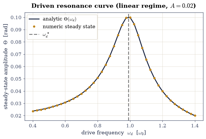
../../_images/b2672b8b4fb8c35ebc2eae80fe4089638d1746b2ce5b277bf92e1e10882a3ebe.png

✓  steady-state amplitude matches the linear resonance curve   [max|Δ| = 1.16715e-05 (rtol=0.02, atol=1e-09)]

True

Exercise 5 — Resonance peak location#

The resonance curve Eq. 106 does not peak at the natural frequency: damping pulls the maximum down to $\omega_d^\star$ given by Eq. 107. The sweep from Exercise 4 already contains the data to test this.

The Exercise-4 grid is too coarse to resolve the small (~1%) shift, so refine the sweep near the peak with the steady_amplitude you wrote in Exercise 4 and find the drive frequency that maximises the response (numpy.argmax).
Confirm it sits at $\omega_d^\star$ of Eq. 107, slightly below the natural frequency.

numeric peak at ω_d = 0.990   analytic ω_d* = 0.990

✓  resonance peaks at √(1-1/2q²)   [got 0.99 vs expected 0.989949 (rtol=1e-06, atol=0.05)]

True

Exercise 6 — Period-doubling cascade (bifurcation diagram)#

Now leave the linear world behind: drive Eq. 103 hard enough that $\sin\theta$ can no longer be linearised, and the tidy resonance picture Eq. 106 fails. The route the system takes to chaos is a period-doubling cascade, and a stroboscopic (Poincaré) sample makes it visible.

Fix $q=2$, $\omega_d=2/3$ and sweep the drive amplitude $A$ across $[1.35, 1.5]$.
Write strobe(A, ...): for a given $A$ it integrates past the transient (scipy.integrate.solve_ivp) and strobes the motion, returning the state sampled once per drive period $T = 2\pi/\omega_d$ — a Poincaré section. Write this one yourself — sampling in step with the drive is what turns a tangled trajectory into a readable picture, and Exercise 7 reuses it for the strange attractor.
Plot the strobed angle against $A$ and read off the cascade: one band splits to two, then four, then dissolves into the broad smear of chaos.

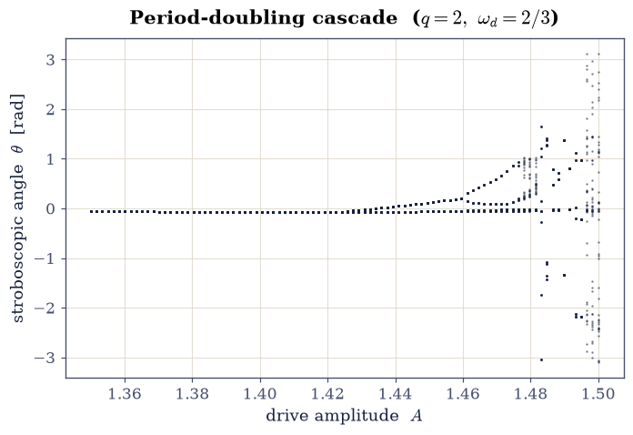
../../_images/fd6a9e06e765ea817d7c30aa1e38a7ced646c17c70f67e6b10790f7f0d172d2d.png

✓  response is more complex at higher drive   [strobe spread: A=1.5 → 2.510  vs  A=1.35 → 0.000]

True

Exercise 7 — Chaos: sensitive dependence at the canonical parameters#

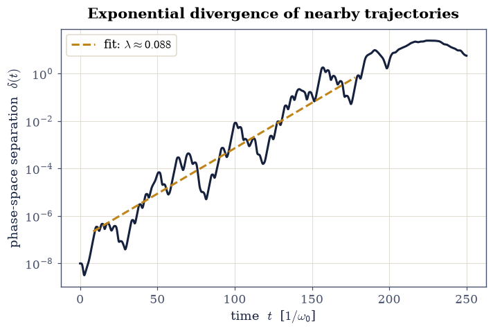
At the canonical chaotic parameters $q=2$, $A=1.5$, $\omega_d=2/3$, Eq. 103 has no periodic steady state at all: the motion is chaotic. The formal signature is sensitive dependence: two nearby starts separate exponentially, $\delta(t)\sim\delta_0 e^{\lambda t}$, with a positive largest Lyapunov exponent $\lambda$.

Settle a reference trajectory onto the attractor with scipy.integrate.solve_ivp, then launch a second differing by $\delta_0 = 10^{-8}$ in angle, running both through your Exercise 2 integrate.
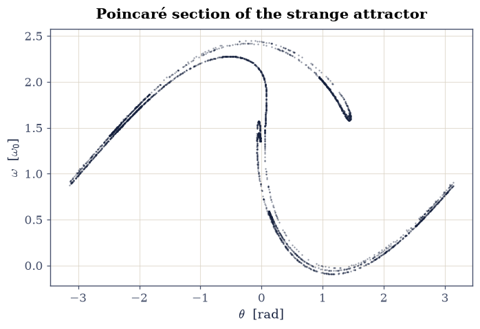
Fit the slope of $\ln\delta(t)$ in its exponential-growth window (numpy.polyfit) to estimate $\lambda$.
Animate the chaotic bob (worked below) and view the strange attractor as a Poincaré section, taking its points from the strobe you wrote in Exercise 6; the final check confirms $\lambda > 0$.

../../_images/760ba7350ff31d87297b1205a035268a465ef21d5b0e412d217bf2ea8dd37b85.png

A Poincaré section (the strobe points of a single long chaotic run) fills out the strange attractor the trajectories are confined to.

../../_images/da2f393bcf7254cd2e99d17583c1a7bf15837a6dadca3a7293d03db916e0c391.png

A worked animation — the chaotic bob#

The Poincaré section is the chaos seen stroboscopically; the animation is the chaos seen continuously. We carry the already-settled base state forward a few dozen drive periods, map the angle to the physical bob position $(x,y) = (\sin\theta, -\cos\theta)$, and watch the rod swing, loop over the top, and never repeat. This is the worked example for the two-animation rule; you build the second one in Exercise 8.

Fig. 85 Animation of the chaotic bob in the strange-attractor regime (quality factor $q=2$, drive amplitude $A=1.5$, drive frequency $\omega_d=2/3$ in units of the natural frequency $\omega_0$): the grey rod links the pivot to the bob at $(x,y)=(\sin\theta,-\cos\theta)$ and the red trail records the never-repeating swing.#

✓  largest Lyapunov exponent is positive (chaotic)   [value = 0.0882044]

True

Exercise 8 — Animate the damped free decay#

This is the second animation, and it is yours to build. We return to the linear-limit physics of Exercise 3: an undriven, underdamped swing whose amplitude decays under the envelope $e^{-t/(2q)}$. The check at the end is physical rather than cosmetic — it reads the decay rate off the animated data and compares it to the $1/(2q)$ of Eq. 104, so it validates what is on screen and not the FuncAnimation object.

Integrate the undriven pendulum at $q=4$ from $\theta_0 = 0.2$ with your Exercise 2 integrate (DOP853 on a fine, dense t_eval), long enough for several oscillations to decay visibly.
Animate $\theta(t)$ advancing under the dashed envelope $\pm\theta_0 e^{-t/(2q)}$ with FuncAnimation (subsample to keep the frame count light).
Measure the decay rate from the peaks of the animated trace (the refined_maxima you wrote in Exercise 3); the validation compares it to $1/(2q)$.

Fig. 86 Animation of the undriven, underdamped free decay at quality factor $q=4$ from initial angle $\theta_0=0.2$ rad: the blue trace is $\theta(t)$ riding inside the dashed envelope $\pm\theta_0 e^{-t/2q}$, whose decay rate $1/(2q)$ is recovered from the animated peaks; time is in units of the inverse natural frequency $1/\omega_0$.#

Validation 8 — the animated decay falls at rate 1/(2q)#

The envelope of the animated $\theta(t)$ must shrink at the rate $1/(2q)$ set by Eq. 104. The check reads the decay rate fitted from the animated trace’s peaks, so it validates the physics on screen rather than the FuncAnimation object.

✓  animated decay falls at rate 1/(2q)   [got 0.125002 vs expected 0.125 (rtol=0.002, atol=1e-09)]

True

With your assistant

The animation scaffolding of Exercise 8 — figure sizing, FuncAnimation wiring, axis dressing — is exactly the kind of code to delegate outright: ask your assistant for it and spend the time on the physics. The check stays yours, and it is physical: the animated decay must halve its amplitude on the timescale your Exercise 3 fit measured.

Notebook summary#

The pendulum equation integrated across regimes: the small-angle period $2\pi/\omega_0$, damped free decay with envelope $\sim e^{-t/2q}$, and the driven resonance peak at $\omega=\omega_0\sqrt{1-1/2q^2}$.
The route to chaos: a period-doubling cascade (bifurcation diagram) and sensitive dependence at the canonical parameters, confirmed by a positive largest Lyapunov exponent.

Outlook#

Basins of attraction. In the multistable (non-chaotic) driven regime, different initial conditions settle onto different periodic attractors. Map which start ends up where and colour the basins.
The full bifurcation diagram. Extend the $A$-sweep over a wider range, resolve several period-doublings, and estimate the Feigenbaum ratio of successive bifurcation spacings.
Integrator choice. Compare RK45 against a symplectic-with-forcing scheme on very long stroboscopic runs: does the attractor’s fine structure survive?

References#

[Nol16]

Wolfgang Nolting. Theoretical Physics 1: Classical Mechanics. Springer, 2016. Grundkurs Theoretische Physik 1.

[Str15]

Steven H. Strogatz. Nonlinear Dynamics and Chaos. Westview Press, 2 edition, 2015.

Take this notebook with you

Use the download button (↓) in the toolbar above to save this notebook and run it yourself. The published notebooks ship without worked solutions; if you would like the reference solutions — to teach from or to check your own work — get in touch: hello@ramador.me.