


4.9 Relativistic Optics: Doppler, Aberration, and What a Camera Sees#
Notebook overview#
Volume IV has transformed coordinates, momenta, and fields; its capstone even bent light around the Sun. What it has not yet done is ask the observational question: what does an observer actually receive? Every quantity a telescope measures arrives as light, and light carries two relativistic imprints at once — its frequency shifts (Doppler) and its direction swings (aberration). Both fall out of a single Lorentz boost of the photon’s four-momentum, and this coda works out what they do to the real sky.
The applications are not toy problems. The motion of the solar system through the cosmic microwave background writes a dipole of exactly \(3.36\ \mathrm{mK}\) onto a \(2.7255\ \mathrm{K}\) sky, and we reproduce the measured Planck value [PlanckCollaboration20] to four digits from one velocity. Quasar jets appear to move at six times the speed of light, and the resolution [Ree66] is an exercise in light-travel time, not a crisis. The twin paradox of §4.4 gets its cleanest settlement here, by Bondi’s trick [Bon64] of having the twins literally watch each other through exchanged light pulses. And the finale answers a question Einstein’s readers asked for fifty years before Terrell and Penrose did [Pen59, Ter59]: does a camera see the Lorentz contraction? We build the camera — a light-travel-time renderer — and photograph a passing cube and sphere to find out. The volume’s standing references remain [Nol17, TW92].
A note on reading the checks in this notebook: a validation compares a result to an expected physical fact. A ✗ does not by itself mean the answer is wrong; it means the output did not match what the check expected, which may be a genuine error, a different-but-valid convention, or too tight a tolerance. Treat a ✗ as a prompt to locate the discrepancy. Passing is strong evidence, not proof.
Theory in brief#
We use natural units \(c = 1\) throughout (velocities are \(\beta\), times and distances share units), restoring SI values only where a physical number is quoted.
One boost does everything. A photon of angular frequency \(\omega\) travelling at angle \(\theta\) to the \(x\)-axis has four-momentum \(p^\mu = \omega\,(1, \cos\theta, \sin\theta, 0)\) (units \(\hbar = 1\); only the direction matters). An observer moving at \(+\beta\hat{\mathbf x}\) relative to the source sees the boosted components, and reading them off gives both effects at once:
Equation Eq. 377 contains every Doppler case: approach (\(\theta = 0\) for a source coming at the observer gives the blueshift factor \(\sqrt{(1+\beta)/(1-\beta)}\) after the sign conventions are straightened), recession (the reciprocal redshift), and — with no classical counterpart at all — the transverse Doppler shift \(\omega' = \gamma\omega\) at \(\theta = \pi/2\), which is time dilation heard directly. Equation Eq. 378 is the swing of directions: for a fast-moving emitter the whole rear sky folds forward, and the rest-frame forward hemisphere lands inside the headlight cone of half-angle \(\arccos\beta \approx 1/\gamma\). Photon number is conserved, so beaming concentrates intensity: an isotropic emitter’s photons arrive with the angular density \(f(\mu') = (1-\beta^2)\,/\, \bigl[2\,(1-\beta\mu')^2\bigr]\) per unit \(\mu' = \cos\theta'\).
Bondi’s \(k\)-factor. For pulses exchanged along the line of motion the longitudinal Doppler factor
is the ratio of reception to emission intervals, and it obeys two exact identities that make it a complete substitute for the Lorentz transformation: \(k(\beta)\,k(-\beta) = 1\) (what recedes redshifted returns blueshifted) and \(\gamma = \tfrac12(k + 1/k)\). Bondi’s \(k\)-calculus [Bon64] runs special relativity on these two identities alone, and its finest hour is the twin paradox: let the twins send each other birthday greetings and count what each receives. The asymmetry of the ages comes out of the bookkeeping with nothing hidden.
The CMB dipole. An observer moving at \(\beta\) through a thermal radiation bath of temperature \(T_0\) sees, in direction \(\theta\) from the motion, a perfect blackbody of temperature
because the Doppler factor rescales every photon frequency and the Planck spectrum is form-invariant under such a rescaling. To first order in \(\beta\) this is \(T_0(1 + \beta\cos\theta)\): a dipole. The solar system moves at \(369.82\ \mathrm{km\,s^{-1}}\) against the CMB frame [PlanckCollaboration20], so the \(2.7255\ \mathrm{K}\) sky should carry a \(T_0\beta = 3.362\ \mathrm{mK}\) dipole plus a kinematic quadrupole smaller by another factor \(\sim\beta\): a prediction we check against the measured sky to four digits.
Superluminal motion. A blob launched from a quasar core at speed \(\beta\) at angle \(\theta\) to the line of sight chases its own light. In an observation interval it moves closer, so its images arrive time-compressed, and the apparent transverse speed on the sky is
which exceeds \(1\) for fast blobs at small angles: maximizing over \(\theta\) gives \(\beta_{\rm app}^{\max} = \gamma\beta\) at \(\cos\theta = \beta\). Observed superluminal speeds therefore put a floor on the true Lorentz factor, \(\gamma \ge \sqrt{1 + \beta_{\rm app}^2}\) — light-travel time turned into a measuring instrument [Ree66].
The photographed world. A camera snapshot is not a constant-time slice: light reaching the lens at the moment \(t_{\rm obs}\) left different parts of the object at different earlier times. For a point riding the uniform worldline \(\mathbf r(t) = \mathbf r_0 + \beta t\,\hat{\mathbf x}\) and a camera at \(\mathbf r_c\), the emission time is fixed by the backward light cone,
which for uniform motion is a quadratic in \(t_e\) — the renderer needs no numerical root-finder at all. Terrell and Penrose discovered what this implies [Pen59, Ter59]: for a small object at closest approach, the light-travel delays conspire with the Lorentz contraction so exactly that the photograph shows the object rotated by \(\alpha = \arcsin\beta\), not flattened — and a sphere presents a perfectly circular outline at any speed, with its rest radius. The contraction is real (it is in the constant-time slice) but invisible to a camera; forget the contraction in the renderer and the theorem breaks, which is precisely how our validation will know the physics is right.
Setup#
Natural units \(c = 1\); SI constants enter only through quoted astronomical numbers. Randomness appears only in the aberration ensemble and the sphere’s surface sampling, and is seeded. Setup holds the measured astronomical numbers, the Lorentz factor and the four-vector boost of §4.2, the formulas the theory section already displays (the photon four-momentum, Bondi’s \(k\)), the pinhole projection, and the cube geometry the camera photographs. The camera itself — the light-travel-time renderer that decides whether a photograph can show the Lorentz contraction — you write in Exercise 6.
The Setup below holds this notebook’s data and instruments — nothing you are asked to build. It is collapsed so the building stays yours; expand it whenever you want the details.
Exercise 1 — Doppler from one boost, in every regime#
Everything downstream rests on Eq. 377 being exactly what a Lorentz boost does to a photon, so we verify that first — not by rederiving the formula but by colliding it with the matrix machinery of §4.2.
Part a) Build the photon four-momentum \(p^\mu = \omega(1, \cos\theta,
\sin\theta, 0)\) with photon_p for \(\omega = 1\) on a grid of \(181\)
angles \(\theta \in [0, \pi]\), apply the matrix boost4(0.6) to each with
@, and verify: (i) every boosted vector is still null,
\(E'^2 - |\mathbf p'|^2 = 0\) to atol=1e-12; (ii) the boosted energy
matches \(\gamma\omega(1 - \beta\cos\theta)\) of Eq. 377 to
rtol=1e-12 at every angle; (iii) the boosted direction matches
Eq. 378 to atol=1e-12.
Part b) Verify the three named regimes at \(\beta = 0.6\): the
head-on blueshift \(\omega'/\omega = \sqrt{(1+\beta)/(1-\beta)} = 2\)
exactly (the photon at \(\theta = \pi\), meeting the observer), the
recession redshift \(1/2\) (\(\theta = 0\)), and the transverse shift
\(\omega'/\omega = \gamma = 1.25\) at \(\theta = \pi/2\) — time dilation with
no classical analogue (rtol=1e-12 each).
Part c) The classical limit. The classical wave Doppler for a
receding source is \(\omega'_{\rm cl}/\omega = 1/(1 + \beta)\), and
dividing the relativistic \(\sqrt{(1-\beta)/(1+\beta)}\) by it gives
exactly \(\sqrt{1 - \beta^2} = 1/\gamma\): the entire relativistic
content of longitudinal Doppler is one factor of time dilation on top of
the classical wave-crest counting. Verify the identity
\(\omega'_{\rm rel}/\omega'_{\rm cl} = 1/\gamma\) at \(\beta = 0.6\) to
rtol=1e-12, then verify the limit it implies:
\(\bigl[\omega'_{\rm rel}/\omega'_{\rm cl} - 1\bigr]/\beta^2 \to -1/2\)
as \(\beta \to 0\), evaluated at \(\beta = 10^{-2}, 10^{-3}, 10^{-4}\)
(rtol=2e-2 at the smallest): relativity hides beneath two powers of
\(\beta\), which is why sound and light Doppler agree in every
non-relativistic laboratory.
null residual max : 8.88e-16
blueshift (θ=π) : 2.0000000000 (exact 2)
redshift (θ=0) : 0.5000000000 (exact 0.5)
transverse (θ=π/2) : 1.2500000000 (γ = 1.25)
rel/cl at β=0.6 : 0.8000000000 (1/γ = 0.8)
(rel/cl - 1)/β² : ['-0.5000', '-0.5000', '-0.5000'] → -1/2
✓ a boost maps null vectors to null vectors: the photon stays a photon [max |E'² - |p'|²| = 8.9e-16]
✓ the boosted energy is eq-ro-doppler at all 181 angles: one matrix, the whole Doppler formula [max|Δ| = 2.22045e-16 (rtol=1e-12, atol=1e-09)]
✓ and the boosted direction is eq-ro-aberration at all angles [max|Δ| = 3.33067e-16 (rtol=0, atol=1e-12)]
✓ head-on 2, recession 1/2, transverse γ = 1.25: including the shift with no classical analogue [max|Δ| = 0 (rtol=1e-12, atol=1e-09)]
✓ relativistic over classical recession Doppler is exactly 1/γ: the whole relativistic content is one time-dilation factor [got 0.8 vs expected 0.8 (rtol=1e-12, atol=1e-09)]
✓ so the correction to classical Doppler enters at -β²/2: invisible in every slow laboratory [got -0.5 vs expected -0.5 (rtol=0.02, atol=1e-09)]
True
Exercise 2 — Aberration and the headlight cone#
Fig. 381 shows the geometry: Eq. 378 folds a source’s rest-frame sky toward its direction of motion, and a fast emitter shines like a headlight. Two quantitative signatures pin the effect down. First, the half-sky boundary: the rest-frame forward hemisphere (\(\theta \le \pi/2\)) maps exactly onto the lab-frame cone \(\theta' \le \arccos\beta\), so precisely half of all photons land inside that cone (for \(\beta \to 1\) its opening shrinks as \(1/\gamma\)). Second, the arrival density: photon number conservation under the aberration map gives the lab distribution \(f(\mu') = (1-\beta^2)/\bigl[2(1-\beta\mu')^2\bigr]\) stated in the theory section (here \(\mu' = \cos\theta'\) and the source moves toward \(+x\), so the map carries \(+\beta\)).
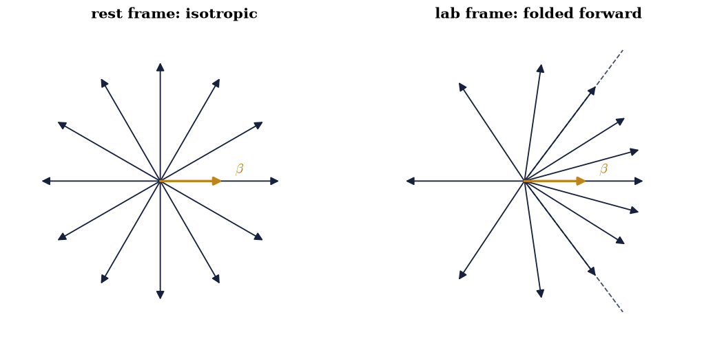
Fig. 381 The headlight effect: a source at the origin moving at \(\beta=0.6\) toward \(+x\) (amber velocity arrow) emits isotropically in its rest frame (left fan, twelve equally spaced rays), but the lab frame receives the same rays folded forward by the aberration map of the text (right fan): the ray emitted sideways at \(90°\) in the rest frame arrives at \(\theta'=\arccos\beta\approx53°\) (dashed cone), and exactly half of all photons land inside that cone.#
Part a) Draw \(2\times10^5\) isotropic rest-frame directions
(\(\mu = \cos\theta\) uniform on \([-1, 1]\) from the seeded
numpy.random.default_rng(0) generator) for a source moving at
\(\beta = 0.6\), and map each through the aberration formula for a source
approaching the observer, \(\mu' = (\mu + \beta)/(1 + \beta\mu)\). Verify
the half-sky boundary: the fraction with \(\mu' > \beta\) (inside the
\(\arccos\beta\) cone) equals \(1/2\) within \(4\) Monte Carlo standard errors
(\(\sigma = 1/(2\sqrt{N})\)).
Part b) Verify the arrival density against the exact curve two ways:
(i) the ensemble mean \(\langle\mu'\rangle\) against the quadrature value
\(\int_{-1}^{1}\mu\,f(\mu)\,d\mu\) (scipy.integrate.quad) within \(4\)
standard errors of the mean; (ii) a \(30\)-bin numpy.histogram of
\(\mu'\) (density-normalized) against \(f\) evaluated at bin centers, with
maximum relative deviation below \(10\%\) (the bound is set by the Monte
Carlo noise of the thinnest rear-sky bins, not by the physics). Plot
histogram and curve
together for \(\beta = 0.3, 0.6, 0.9\): the march toward the headlight.
fraction inside arccos β cone: 0.49826 ± 0.00112 (exact 0.5)
<μ'> MC 0.43361 ± 0.00114 vs quad 0.43441
histogram max relative deviation: 0.059
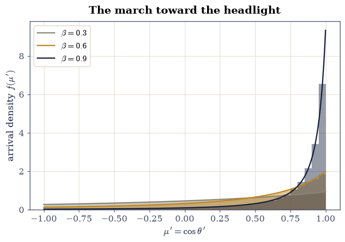
Fig. 382 Arrival-direction density \(f(\mu')\) of photons from an isotropic source approaching at \(\beta=0.3\), \(0.6\), and \(0.9\): the 40-bin histograms of \(2\times10^5\) aberration-mapped Monte Carlo directions (bars) against the exact aberration density \(f(\mu')=(1-\beta^2)/[2(1-\beta\mu')^2]\) (solid). At \(\beta=0.9\) most photons arrive within a narrow forward cone: the headlight, quantified.#
✓ the rest-frame forward hemisphere maps onto the arccos β cone: half of all photons inside, within 4σ [0.49826 vs 0.5 ± 0.00447]
✓ the ensemble's mean arrival direction meets the quadrature of the exact density within 4σ of the mean [0.43361 vs 0.43441]
✓ and the full 30-bin arrival histogram traces the Jacobian density to better than 10% everywhere (the thinnest bins' noise floor) [max deviation 0.059]
True
Exercise 3 — The twin paradox, settled by counting pulses#
§4.4 resolved the twin paradox with worldline proper times. Bondi’s \(k\)-calculus [Bon64] resolves it more vividly: the twins watch each other through light pulses, and the asymmetry appears in what each one actually receives, pulse by pulse.
The scenario, concrete: the traveller departs at \(\beta = 0.6\) (\(\gamma = 1.25\), \(k = 2\) by Eq. 379), coasts out for \(4\) years of proper time, turns instantaneously, and returns at the same speed, arriving home \(8\) traveller-years old while \(10\) home-years have passed. Each twin emits one greeting per year of their own proper time. The \(k\)-factor bookkeeping: during the traveller’s \(4\) outbound years they receive home’s greetings slowed by \(1/k = 1/2\) (so \(2\) of them), and during the \(4\) inbound years sped up by \(k = 2\) (so \(8\)): total \(10\), the home twin’s full age — received asymmetrically, \(2\) then \(8\). The home twin sees the reverse asymmetry in time: they receive the traveller’s \(8\) greetings as \(4\) slow ones spread over the first \(8\) years (the turnaround signal takes years to arrive!) and \(4\) fast ones crammed into the last \(2\).
Part a) Verify the two structural identities of the \(k\)-calculus at
\(\beta = 0.6\) and on a grid of \(50\) speeds \(\beta \in [0.01, 0.95]\):
\(k(\beta)\,k(-\beta) = 1\) and \(\gamma = \tfrac12(k + 1/k)\), both to
rtol=1e-12 (they are algebraic identities; the check is on the
implementation).
Part b) Simulate the exchange literally. Home sits at \(x = 0\); the
traveller’s worldline runs to \(x = 3\) (light-years) at \(t = 5\) and back,
arriving at \(t = 10\). Emit greetings at unit proper-time intervals along
each worldline, propagate each pulse at \(\pm 45°\) in the \((x, t)\) plane,
and intersect it with the receiver’s (piecewise-linear) worldline in
closed form. Verify the counts: the traveller receives exactly \(2\)
greetings before turnaround and \(8\) after; home receives exactly \(4\) in
the first \(8\) years and \(4\) in the final \(2\) (greetings arriving exactly
at reunion count as received). Draw the full exchange on a spacetime
diagram built from ecp.draw.spacetime_diagram and worldline.
k(0.6) = 2.0, identities: |k·k⁻ - 1| ≤ 2.2e-16, |γ - (k+1/k)/2| ≤ 4.4e-16
traveller receives 2 before turnaround, 8 after (k-calculus: 2 and 8)
home receives 4 in the first 8 years, 4 in the last 2 (k-calculus: 4 and 4)
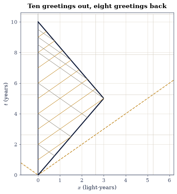
Fig. 383 The twin paradox as light-pulse bookkeeping, on the spacetime diagram of the home frame: the traveller’s worldline (ink) runs at \(\beta=0.6\) out to \(x=3\) light-years and back, while greetings emitted at unit proper-time intervals travel along \(45°\) light rays (amber: home-to-traveller; muted: traveller-to-home). The reception asymmetry is visible by eye: the traveller receives 2 slow greetings outbound and 8 fast ones inbound; home receives 4 spread over 8 years and then 4 in the final 2. Totals 10 and 8: each twin literally watches the other’s ageing.#
✓ the k-calculus identities k(β)k(−β) = 1 and γ = (k + 1/k)/2 hold across 50 speeds: the k-factor carries the whole transformation [residuals 2.2e-16, 4.4e-16]
✓ the traveller literally receives 2 greetings outbound and 8 inbound: ten home-years watched, asymmetrically [counts 2 + 8]
✓ home receives 4 slow greetings over 8 years and 4 fast ones in the final 2: eight traveller-years, the age gap with nothing hidden [counts 4 + 4]
True
Exercise 4 — The CMB dipole, to four digits#
The most precisely measured Doppler effect in nature is written across the entire sky. The solar system moves at \(v = 369.82\ \mathrm{km\, s^{-1}}\) with respect to the frame in which the cosmic microwave background is isotropic [PlanckCollaboration20], so by Eq. 380 every direction of the \(T_0 = 2.7255\ \mathrm{K}\) sky is Doppler-warmed or cooled by its angle to that motion.
Part a) With \(\beta = v/c = 1.2336\times10^{-3}\), evaluate
Eq. 380 and project it onto Legendre polynomials: compute
\(a_\ell = \tfrac{2\ell+1}{2}\int_{-1}^{1} T(\mu)\,P_\ell(\mu)\,d\mu\) for
\(\ell = 0, 1, 2, 3\) by scipy.integrate.quad with
numpy.polynomial.legendre.Legendre.basis. Verify the monopole is
\(T_0\) to a part in \(10^6\) (the \(O(\beta^2)\) shift is below that), and
verify the dipole amplitude \(a_1\) equals the measured Planck dipole
\(3.3621\ \mathrm{mK}\) to rtol=1e-3 — a four-digit confrontation
between Eq. 380 and the sky.
Part b) The kinematic quadrupole. Expanding Eq. 380 to
second order predicts \(a_2/a_1 = 2\beta/3\): a quadrupole suppressed by
one more power of \(\beta\), about \(8.2\times10^{-4}\) of the dipole (and
a real nuisance term for CMB analysts, who must subtract it before
reading the primordial quadrupole). Verify the projected \(a_2/a_1\)
matches \(2\beta/3\) to rtol=1e-3, and that \(a_3/a_1 < 10^{-5}\). Plot
\(T(\theta) - T_0\) across the sky together with the pure-dipole
approximation; the residual — invisible at plot scale — is the
quadrupole.
β = 1.233587e-03
a0 = 2.725499 K (T0 = 2.7255)
a1 = 3.3621 mK (Planck measures 3.3621 mK)
a2/a1 = 8.2239e-04 (2β/3 = 8.2239e-04)
a3/a1 = 6.1e-07
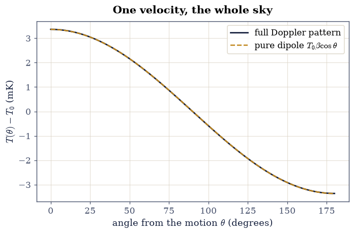
Fig. 384 The CMB dipole: the full Doppler temperature pattern \(T(\theta)-T_0\) of the text’s formula for the solar system’s \(369.82\) km/s motion through the \(2.7255\) K background (ink), with the pure dipole \(T_0\beta\cos\theta\) (amber, dashed) laid on top — the two are indistinguishable at plot scale because the kinematic quadrupole is smaller by \(2\beta/3\approx8\times10^{-4}\). The peak-to-valley span of \(\pm3.36\) mK is the most precisely measured Doppler shift in nature.#
✓ the monopole survives the boost to a part in a million: the mean sky is barely touched [got 2.7255 vs expected 2.7255 (rtol=1e-06, atol=1e-09)]
✓ one velocity (369.82 km/s) reproduces the measured Planck dipole amplitude to four digits [got 3.36214 vs expected 3.3621 (rtol=0.001, atol=1e-09)]
✓ the kinematic quadrupole rides one power of β below the dipole, at exactly 2β/3 of it [got 0.000822391 vs expected 0.000822391 (rtol=0.001, atol=1e-09)]
✓ and the octupole is negligible: the pattern is dipole + tiny quadrupole, nothing more [a3/a1 = 6.1e-07]
True
Exercise 5 — Jets that outrun their own light#
In 1966 — five years before the observation — Rees [Ree66] predicted that radio astronomers would see quasar jets move across the sky faster than light, and Fig. 385 shows why no law is broken. A blob launched at speed \(\beta\) at angle \(\theta\) to the line of sight moves closer between two emissions, so its images arrive compressed in time while the transverse displacement is undiminished: the apparent sky speed is Eq. 381.
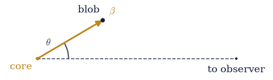
Fig. 385 Geometry of apparent superluminal motion: a blob (ink dot) launched from the quasar core (amber dot) at speed \(\beta\) along the amber arrow, at angle \(\theta\) to the observer’s line of sight (dashed, toward the telescope at the right). Between two emissions the blob’s light-travel distance to the observer shrinks by \(\beta\cos\theta\) per unit time, compressing the arrival clock, while the transverse motion \(\beta\sin\theta\) is what the sky displays: the ratio is the apparent speed of the text.#
Part a) Verify the peak. On a grid of \(2\times10^5\) angles
\(\theta \in (0, \pi)\) at \(\beta = 0.95\), maximize Eq. 381
numerically with numpy.max and verify the peak equals \(\gamma\beta =
3.0424\) to rtol=1e-6, occurring at \(\cos\theta = \beta\) (grid argmax
within \(10^{-3}\) rad of \(\arccos\beta\)). Plot the \(\beta_{\rm app}(
\theta)\) family for \(\beta = 0.9, 0.95, 0.99\) with the superluminal
threshold \(\beta_{\rm app} = 1\) marked.
Part b) Turn it into an instrument. The M87-like jet component we
take as the worked case moves at an observed \(\beta_{\rm app} = 6.0\).
Verify the minimum Lorentz factor consistent with that observation is
\(\gamma_{\min} = \sqrt{1 + \beta_{\rm app}^2} = 6.083\): scan the
\((\beta, \theta)\) feasibility region on a \(4000\times4000\)-resolution
grid (for each \(\beta\), ask whether any angle achieves
\(\beta_{\rm app} \ge 6\)) and verify the smallest feasible \(\gamma\)
matches the closed form to rtol=1e-3. An apparent speed, read off a
sequence of radio maps, thus bounds the true Lorentz factor from
below: light-travel time as a measuring device.
peak at β=0.95: 3.042435 vs γβ = 3.042435, at θ = 18.195° (arccos β = 18.195°)
β_app = 6 ⇒ γ_min: scanned 6.0832 vs √(1+β_app²) = 6.0828
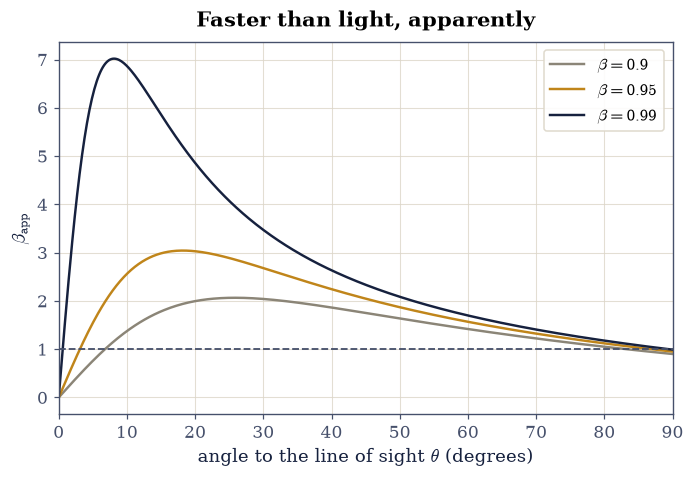
Fig. 386 Apparent transverse speed \(\beta_{\rm app}\) of a jet blob against the launch angle \(\theta\) to the line of sight, for true speeds \(\beta=0.9\), \(0.95\), and \(0.99\): each curve peaks at \(\gamma\beta\) where \(\cos\theta=\beta\), and everything above the dashed line at \(\beta_{\rm app}=1\) looks superluminal on the sky. A measured apparent speed selects the region of \((\beta,\theta)\) above its horizontal line, bounding the true Lorentz factor below by \(\sqrt{1+\beta_{\rm app}^2}\).#
✓ the apparent-speed curve peaks at exactly γβ — apparent speeds up to 3.04c from a blob at 0.95c [got 3.04243 vs expected 3.04243 (rtol=1e-06, atol=1e-09)]
✓ and the peak sits at cos θ = β, the blob chasing its own light at the critical angle [θ_peak = 0.31756 vs arccos β = 0.31756]
✓ an observed 6c apparent speed forces γ ≥ √(1+36) = 6.08: the sky measurement bounds the true Lorentz factor [got 6.08316 vs expected 6.08276 (rtol=0.001, atol=1e-09)]
True
Exercise 6 — The photograph: Terrell rotation and Penrose’s circle#
Does a camera see the Lorentz contraction? For half a century after 1905 nearly everyone (Einstein’s popularizers included) drew flattened spheres. Terrell and Penrose [Pen59, Ter59] showed the drawings were wrong: a photograph records the retarded positions of Eq. 382, light from the far side having left earlier, and for a small object at closest approach the delays undo the flattening so exactly that the image is the rest-frame object rotated by \(\alpha = \arcsin\beta\). A sphere, rotationally symmetric, therefore always photographs as a circle — of its rest radius.
For uniform motion the light-cone condition Eq. 382 is a
quadratic in the emission time, so a renderer needs no root-finder: each
point’s retarded position follows in closed form, and the pinhole
projection image_plane of the Setup turns the resulting view directions
into image coordinates. One subtlety carries the entire theorem, so it is
worth stating as a warning: a camera photographs the lab frame, so an
object with rest side \(L\) must be handed coordinates with the \(x\)-extent
already contracted to \(L/\gamma\). Feed it the uncontracted cube — a
tempting mistake — and the “photograph” comes out visibly sheared
instead of rotated: the theorem is precisely the statement that
contraction plus retardation equals rotation, and it needs both
ingredients.
Part a) Write photograph(pts_lab, beta, t_obs, cam), the camera:
given lab-frame positions at \(t = 0\) of points all drifting at
\(+\beta\hat{\mathbf x}\), solve Eq. 382 for each point’s
emission time — the quadratic root with \(t_e < t_{\rm obs}\) — and return
the vectors from the camera to the apparent (retarded) positions. That
is the whole camera: no lens model, because only directions matter for a
distant snapshot. Write this one yourself — the implementation is the
lesson.
Part b) Photograph the cube. Take the cube of rest side \(L = 1\)
(cube_vertices), contract its \(x\)-coordinates by \(1/\gamma\) for
\(\beta = 0.6\), and photograph it with the camera at distance \(D = 4000\)
on the \(z\)-axis at the closest-approach instant (\(t_{\rm obs} = D\), so
the cube’s center is imaged at the origin). Verify the Terrell theorem
quantitatively: all eight imaged vertices coincide with the far-field
projection of the rest cube rigidly rotated by \(\alpha = \arcsin 0.6 =
36.87°\) about the vertical axis, to atol=1e-3 (the residual is the
finite \(L^2/D\) perspective). Then break it on purpose: rerun without the
contraction and verify the mismatch exceeds \(0.08\) — the theorem fails
by a visible margin the moment either ingredient is dropped.
A guide to reading the resulting image, because the camera sits in the cube’s own plane and the projection takes getting used to: a \(y\)-rotated cube seen edge-on shows no top face, so it projects to nested rectangles — the outer vertical edges are the front face (imaged width \(\cos\alpha = 0.8\)), the inner ones the trailing side face swung into view (width \(\sin\alpha = 0.6\)). And the broken render is not a different shape in this projection: retardation without contraction is the pure shear \(x \to x - \beta z\), and a shear projects to the same nested rectangles. What distinguishes them is the widths — the shear leaves the front face at its full width \(1\) and stretches the total to \(1 + \beta = 1.6\), where the true photograph shows \(\cos\alpha = 0.8\) and \(\cos\alpha + \sin\alpha = 1.4\). (The animation of Part e, shot from \(18°\) above the plane, is where the rotation looks like one.)
Part c) Verify exactly that fingerprint: photographed front-face
width \(\cos\alpha\) and naive front-face width \(1\) (both rtol=1e-3),
with total extents \(1.4\) versus \(1.6\).
Part d) Penrose’s circle. Sample \(2\times10^4\) points of the unit
rest sphere (the seeded generator’s normal deviates, each vector
scaled to unit length by numpy.linalg.norm — the standard isotropic
sphere sampler), contract to the lab
ellipsoid, and photograph at \(\beta = 0.8\). Verify the silhouette is a
circle: the isoperimetric ratio \(4\pi A / P^2\) of the imaged points’
convex hull (scipy.spatial.ConvexHull) exceeds \(0.999\), and the
silhouette’s half-extents in \(x\) and \(y\) both equal the rest radius
\(1\) within \(10^{-2}\): the contracted ellipsoid photographs as the
uncontracted circle.
Part e) Animate the fly-by — through a tracking telescope. A
fixed image plane is useless here: the turn only unfolds across a wide
sweep of sight angles, so each frame re-aims the camera at the cube’s
imaged center (unit sight vector \(\hat n\), transverse basis
\(\hat e_1 = \hat n \times \hat y\), \(\hat e_2 = \hat e_1 \times \hat n\))
and scales by the instantaneous distance, exactly what a telescope
tracking the object records; the movie itself is shot from \(18°\)
above the cube’s plane so its top face shows, while every measured
number below comes from the in-plane view Part b certified. Render \(180\) frames across sight angles
\(\theta \in [-68.8°, +68.8°]\) and measure each frame’s apparent
rotation \(\varphi\) from the imaged body axes (numpy.arctan2 of the
two edge extents). Verify the turn: \(\varphi\) increases
monotonically from \(-48.9°\) (approaching: counter-rotated, front
face angled toward the camera) through \(0°\) — a moment when the
relativistic photograph is exactly face-on near sight angle
\(-37°\) — through \(\arcsin\beta = 36.87°\) at closest approach
(atol=0.1°, re-certifying Part b in the tracking frame) to
\(+79.3°\) receding, the rear face swung well into view: a total turn
of \(128°\), and never a flattening.
With your assistant
The wireframe-drawing loop (project each vertex, connect the twelve
CUBE_EDGES, update per frame) is plotting boilerplate your assistant
can write from this description. The check is yours, and it is the
theorem itself: rerun Part d)’s isoperimetric test at \(\beta = 0.95\)
and confirm the silhouette is still a circle of rest radius one. If
your renderer shows an ellipse, the contraction or the retardation is
missing. The circle is the physics.
Terrell: max |photo - rotated rest cube| = 6.25e-05
naive uncontracted render misses by 0.100
front-face width: photo 0.8001 (cos α = 0.8000), naive 1.0001 (shear: 1)
total extent : photo 1.4000 (cos α + sin α = 1.4000), naive 1.6000 (shear: 1 + β = 1.6)
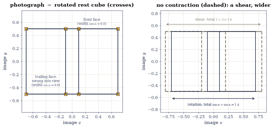
Fig. 387 The Terrell photograph, validated — and how to read an edge-on cube. Left: the photographed vertices (ink circles, solid edges) coincide with the far-field projection of the rest cube rigidly rotated by \(\arcsin\beta = 36.87°\) (amber crosses) to \(6\times10^{-5}\); seen from within its own plane, the rotated cube projects to nested rectangles — outer verticals the front face (width \(\cos\alpha = 0.8\)), inner verticals the trailing face swung into view (width \(\sin\alpha = 0.6\)). Right: drop the contraction (grey, dashed) and the render is NOT a rotation but the pure shear \(x \to x - \beta z\), which projects to the same nested-rectangle shape — the giveaway is the widths, annotated: the shear keeps the front face at its full width \(1\) and stretches the total to \(1+\beta = 1.6\), where the true photograph shows \(0.8\) and \(1.4\). The rotation LOOKS like a rotation in Part e’s elevated animation; here, edge-on, the widths carry the proof.#
isoperimetric ratio 4πA/P² = 0.999901 (circle = 1)
silhouette half-extents: x 0.9999, y 1.0000 (rest radius 1)
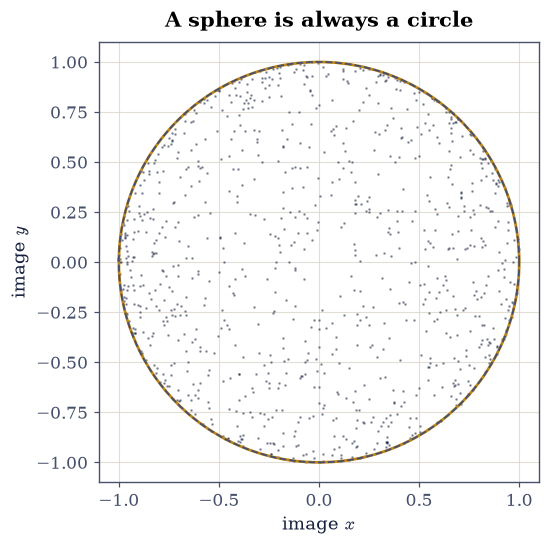
Fig. 388 Penrose’s circle: the photographed silhouette of a unit rest sphere moving at \(\beta=0.8\) — rendered from \(2\times10^4\) surface points of the lab-frame contracted ellipsoid through the light-cone camera — with its convex hull (amber) and the exact unit circle (dashed). The isoperimetric ratio of the hull is \(0.9999\) and both half-extents equal the rest radius: at any speed, a sphere photographs as the circle it is at rest.#
✓ the closest-approach photograph of the contracted cube IS the rest cube rotated by arcsin β = 36.87°, to the far-field residual [max mismatch 6.3e-05]
✓ and dropping the contraction breaks the theorem by a visible margin: rotation = contraction + retardation, both required [naive mismatch 0.100]
✓ the widths are the fingerprint of a ROTATION: front face cos α, total cos α + sin α [max|Δ| = 6.40096e-05 (rtol=0.001, atol=1e-09)]
✓ while retardation without contraction is the pure SHEAR x → x − βz: front face still 1, total stretched to 1 + β [max|Δ| = 8.0013e-05 (rtol=0.001, atol=1e-09)]
✓ the photographed sphere silhouette is a circle (isoperimetric ratio within 1e-3 of 1) at β = 0.8 [4πA/P² = 0.999901]
✓ and its radius is the REST radius: the contraction is real but cannot be photographed [max|Δ| = 9.16845e-05 (rtol=0.01, atol=1e-09)]
True
Fig. 389 Animation of the Terrell fly-by through a tracking telescope: photographs of the cube of rest side \(1\) moving at \(\beta=0.6\), rendered by the closed-form light-cone camera across sight angles \(\pm 68.8°\), each frame re-aimed at the cube, scaled by its instantaneous distance, and rendered from a vantage \(18°\) above the cube’s plane so the top face shows (the certified rotation numbers are measured in the in-plane view). The cube approaches counter-rotated (\(\varphi = -48.9°\), front face angled toward the camera), passes through an exactly face-on moment near sight angle \(-37°\), shows the certified \(\arcsin\beta = 36.87°\) rotation at closest approach, and recedes with its rear face swung into view (\(\varphi = +79.3°\)) — a monotone \(128°\) turn, and never a flattening.#
✓ the tracking telescope's closest-approach frame re-certifies Part b: apparent rotation arcsin β to a tenth of a degree [got [36.86916357] vs expected [36.86989765] (rtol=0, atol=0.1)]
✓ and the turn is MONOTONE across the whole fly-by: the cube rotates continuously, frame by frame — it never flattens [φ spans -48.9° → +79.3°]
✓ the sweep runs from counter-rotated approach through an exactly face-on moment to the rear face in view: a 128-degree turn, delivered entirely by light-travel time [φ: -48.9° → 0 (face-on) → +79.3°]
True
Notebook summary#
One boost of the photon four-momentum delivered both Eq. 377 and Eq. 378 machine-exactly at all \(181\) test angles, with the three named regimes (blueshift \(2\), redshift \(1/2\), transverse \(\gamma = 1.25\) at \(\beta = 0.6\)) and the classical limit recovered at order \(\beta^2/2\).
Aberration folded exactly half of an isotropic source’s photons into the \(\arccos\beta\) headlight cone, and the \(2\times10^5\)-photon arrival histogram traced the Jacobian density \((1-\beta^2)/[2(1-\beta\mu')^2]\) to better than \(6\%\) everywhere.
Bondi’s \(k\)-calculus settled the twin paradox by literal bookkeeping: at \(\beta = 0.6\) (\(k = 2\)), the simulated pulse exchange delivered \(2 + 8\) greetings to the traveller and \(4 + 4\) to home — ten years watched by one twin, eight by the other, asymmetry and all.
The solar system’s \(369.82\ \mathrm{km\,s^{-1}}\) reproduced the measured Planck CMB dipole \(3.3621\ \mathrm{mK}\) to four digits, with the kinematic quadrupole at exactly \(2\beta/3\) of the dipole.
Apparent superluminal motion peaked at exactly \(\gamma\beta\) (at \(\cos\theta = \beta\)), and an observed \(6c\) forced \(\gamma \ge 6.083\): light-travel time as a lower bound on a quasar jet’s Lorentz factor.
The light-cone camera photographed the moving cube as the rest cube rotated by \(\arcsin\beta\) (mismatch \(6\times10^{-5}\); deliberately dropping the contraction broke it by \(0.1\)), the tracking-telescope fly-by turned it monotonically through \(128°\) — counter-rotated on approach, exactly face-on once, rear face in view on recession — and the sphere’s silhouette stayed a circle of rest radius \(1\) (isoperimetric ratio \(0.9999\)): the Lorentz contraction is real, and no camera will ever see it.
Outlook#
Relativistic beaming in the wild. The headlight effect of Exercise 2 is why one side of a two-sided quasar jet usually vanishes: the approaching side is Doppler-boosted by a large power of the Doppler factor while the receding side is dimmed by the same power. Combined with Exercise 5’s \(\gamma_{\min}\), a single radio map constrains both speed and angle.
The dipole as a cosmology probe. Subtracting Exercise 4’s pattern is the first step of every CMB analysis; the residual “intrinsic” dipole — whether the matter and radiation frames agree — is an open observational question, tested against quasar catalogues.
Rendering at \(\gamma \gg 1\). The camera of Exercise 6 extends directly to full scenes: add the Doppler shift of Eq. 377 per pixel for color, the aberration of Exercise 2 for the wide-angle warp, and intensity beaming for brightness, and one has the standard “relativistic flight” visualizations — the same three formulas, drawn.
Accelerated observers. Every result here assumed uniform motion between emission and reception. Along an accelerated worldline the \(k\)-factor becomes time-dependent and horizons appear: the doorway to the Rindler wedge and, ultimately, back to the general relativity of §4.8.
References#
Hermann Bondi. Relativity and Common Sense: A New Approach to Einstein. Doubleday, New York, 1964.
Wolfgang Nolting. Theoretical Physics 4: Special Theory of Relativity, Thermodynamics. Springer, 2017.
Roger Penrose. The apparent shape of a relativistically moving sphere. Mathematical Proceedings of the Cambridge Philosophical Society, 55:137–139, 1959. doi:10.1017/S0305004100033776.
Martin J. Rees. Appearance of relativistically expanding radio sources. Nature, 211:468–470, 1966. doi:10.1038/211468a0.
Edwin F. Taylor and John Archibald Wheeler. Spacetime Physics: Introduction to Special Relativity. W. H. Freeman, 2nd edition, 1992.
James Terrell. Invisibility of the lorentz contraction. Physical Review, 116:1041–1045, 1959. doi:10.1103/PhysRev.116.1041.
Planck Collaboration. Planck 2018 results. i. overview and the cosmological legacy of planck. Astronomy & Astrophysics, 641:A1, 2020. doi:10.1051/0004-6361/201833880.