0.3 Numerical Integration and Differentiation

Elementary Computational Physics

Volume 0 — Mathematical & Computational Foundations Notebook 0.3

Computing integrals and derivatives that cannot be done by hand: the quadrature rules, their convergence orders, Richardson extrapolation, and why raising the order beats shrinking the step.

Level · intermediate   •   Est. · 80–110 min

Raymond Amador v1.4.0  ·  2026-07-31  ·  CC BY 4.0 (text) / MIT (code)

Notebook overview

The mathematical symbols \(\int_a^b f\,dx\) and \(f'(x)\) are familiar to us. Yet the question remains regarding exactly how a computer produces them when there is no antiderivative to write down and no symbol to differentiate, which is almost always, in real physics. The answers are quadrature rules (integrals as weighted sums of samples) and finite- difference stencils (derivatives as weighted differences), and the interesting part is not the formulas but their error behaviour: how fast each converges, and where round-off (§0.1) sets a floor that no smaller step can beat.

The throughline is order. A rule’s convergence order \(p\) (error \(\sim C\,h^p\)) is the single number that decides whether we need ten samples or ten thousand. We will measure \(p\) for the trapezoid, midpoint, and Simpson rules (2, 2, 4); double it for free with Richardson extrapolation; reach the spectacular efficiency of Gaussian quadrature (\(n\) points exact for degree \(2n-1\)); measure the orders of three derivative stencils (1, 2, 4); and close the loop with §0.1: for a smooth function, raising the order beats shrinking the step, because higher order reaches a lower error before round-off takes over.

This points forward: adaptive quadrature (Exercise 8) is the workhorse behind the orbital and scattering integrals of §2.4–§2.5 and the descent-time integral of §2.8. Exercise 9 then attaches the one precondition that makes any of it safe: an adaptive rule must find the integrand before it can refine anywhere, so the physics is scaled to order one first. That is a standing rule of the course, and it belongs here, where quad is met, rather than in Volume VII where its absence first bites. There are no animations here: nothing in this material moves; a convergence plot is best read as a still figure, and that is the right choice.

How to read the checks. Each exercise ends with a validate call against an independent fact: a known integral, a predicted order, an exactness result. A ✓ is strong evidence; a ✗ is a prompt to locate the discrepancy (an even-\(n\) requirement, an order fit on the round-off tail), not a verdict.

Scope. A working review, not a numerical-analysis text. The standard reference is Press et al., Numerical Recipes, ch. 4 [PTVF07]; round-off limits trace back to §0.1 and Higham [Hig02].

Theory in brief

Quadrature: integrals as weighted samples

A quadrature rule approximates \(\int_a^b f\,dx\) by a weighted sum of function values, and the rules differ only in which values and what weights. The simplest family, Newton–Cotes, fixes equally spaced samples \(x_i=a+ih\), \(h=(b-a)/n\), and reads the weights off the polynomial that interpolates them, so a better interpolant gives a better rule. A straight line through the panel endpoints yields the composite trapezoid rule,

(12)\[T(h) = h\left[\tfrac12 f_0 + f_1 + \cdots + f_{n-1} + \tfrac12 f_n\right], \qquad \text{error } = O(h^2);\]

sampling the panel centres instead gives the composite midpoint rule, also \(O(h^2)\) but typically with about half the error, since its over- and undershoots on a convex arc partly cancel:

(13)\[M(h) = h\sum_{i=0}^{n-1} f\!\left(a + (i+\tfrac12)h\right), \qquad \text{error } = O(h^2).\]

Stepping up from a line to a parabola across each pair of panels gives Simpson’s rule, where one extra sample per pair of panels buys a remarkable two orders (all three error terms follow from the Taylor remainder of the interpolating polynomial; Press et al., Numerical Recipes, §4.1, tabulate them in full):

(14)\[S(h) = \frac{h}{3}\left[f_0 + 4f_1 + 2f_2 + 4f_3 + \cdots + 4f_{n-1} + f_n\right], \qquad \text{error } = O(h^4) \quad (n \text{ even}).\]

Order, Richardson, and Gauss

The order \(p\) of a rule is defined by error \(\approx C\,h^p \approx C'\,n^{-p}\),

(15)\[\varepsilon(n) \approx C'\,n^{-p} \quad\Longrightarrow\quad \log\varepsilon \approx \text{const} - p\,\log n,\]

so \(p\) is minus the slope of a log–log error-vs-\(n\) plot. Richardson extrapolation combines two estimates to cancel the leading error term: since trapezoid error is \(\propto h^2\), the combination

(16)\[\frac{4\,T(h/2) - T(h)}{3} = O(h^4)\]

is two orders better for free; iterating this is Romberg integration. (The Euler–Maclaurin formula supplies the underlying \(h^2\) series; Press et al., Numerical Recipes, §§4.2–4.3, develop it and build Romberg from it.) Gaussian quadrature goes further still: by choosing both the nodes and the weights optimally (the nodes are roots of Legendre polynomials), \(n\) points integrate every polynomial of degree \(\le 2n-1\) exactly,

(17)\[\int_{-1}^{1} f(x)\,dx \approx \sum_{i=1}^{n} w_i\,f(x_i), \qquad \text{exact for } \deg f \le 2n-1,\]

and converges spectrally (faster than any fixed power of \(n\)) for smooth \(f\). The exactness theorem rests on the orthogonality of the Legendre polynomials; Press et al., Numerical Recipes, §4.6, give the proof.

Differentiation stencils and the round-off floor

Derivatives combine samples with differencing weights. The forward, central, and fourth-order central stencils are

(18)\[\begin{split}\begin{aligned} f'(x) &\approx \frac{f(x+h)-f(x)}{h} && O(h), \\[2pt] f'(x) &\approx \frac{f(x+h)-f(x-h)}{2h} && O(h^2), \\[2pt] f'(x) &\approx \frac{-f(x+2h)+8f(x+h)-8f(x-h)+f(x-2h)}{12h} && O(h^4). \end{aligned}\end{split}\]

Each row follows from Taylor-expanding \(f(x\pm h)\) about \(x\) and cancelling the unwanted terms; Press et al., Numerical Recipes, §5.7, tabulate the standard stencils. As in §0.1, shrinking \(h\) helps only until round-off in the differenced numerator takes over; past that the error grows. The lever for a smooth function is therefore order, not step: a higher-order stencil reaches a lower error before hitting its round-off floor.

Setup

Data and instruments only: the running test integral \(\int_0^1 e^x\,dx = e-1\) with its closed form, the library imports (scipy.integrate.quad for the adaptive comparison of Exercise 8, numpy.polynomial.legendre.leggauss for the Legendre nodes and weights of Exercise 5), fit_order, a log–log slope diagnostic that reads an empirical convergence order off an error sweep, and the specimen Exercise 9 integrates: CODATA \(\hbar\), \(c\), \(k_B\), the Sun’s effective temperature, and Planck’s law itself, which §7.14 derives and this notebook merely takes as given. Every rule this notebook is about — trapezoid, midpoint, Simpson, Gauss–Legendre, the three difference stencils, and the nondimensionalization that makes Planck’s law integrable — you build in the exercise where it is earned.

The Setup below holds this notebook’s data and instruments — nothing you are asked to build. It is collapsed so the building stays yours; expand it whenever you want the details.

Show code cell source

Hide code cell source

import warnings

import numpy as np
import matplotlib.pyplot as plt
from math import erf
from scipy.integrate import quad
from scipy.constants import hbar as HBAR, c as C, k as KB
from numpy.polynomial.legendre import leggauss

from ecp import validate


# instrument: a diagnostic, not the lesson — the physics here is the rules and
# stencils themselves; reading their order off an error sweep is one
# least-squares line in log space (any library fit would serve identically), and
# it is applied to whatever errors the exercises hand it.
def fit_order(ns, errs):
    """Empirical convergence order p: minus the slope of log(error) vs log(n).

    Parameters
    ----------
    ns : array_like
        Panel counts.
    errs : array_like
        Corresponding errors.

    Returns
    -------
    float
        The estimated order $p$.
    """
    ns, errs = np.asarray(ns, float), np.asarray(errs, float)
    # Exclude points at the round-off floor (0.1): once the error saturates near
    # machine epsilon it no longer follows C·n^(−p), and including those points
    # would drag the fitted slope toward zero.
    m = errs > 1e-13
    return -np.polyfit(np.log(ns[m]), np.log(errs[m]), 1)[0]


# data: smooth test integral used throughout, ∫₀¹ eˣ dx = e − 1 (integrand and
# closed form).
f_exp = np.exp
I_exp = np.e - 1.0

# data: the IAU nominal solar effective temperature, the specimen temperature of
# Exercise 9.
T_SUN = 5772.0  # K


# data: Planck's law for the spectral energy density of blackbody radiation,
# u(ω, T) = ħω³/(π²c³) · 1/(e^{ħω/k_BT} − 1). Derived in §7.14 and handed over
# here as a given integrand — Exercise 9's lesson is the SCALING, not the physics.
# The denominator goes through numpy.expm1 for the reason §0.1 gives.
def u_planck(w, T):
    """Planck spectral energy density u(ω, T), SI units of J·s/m³.

    The given specimen of Exercise 9: ordinary physics whose SI scales (a peak near
    ω ≈ 2×10¹⁵ rad/s, a height near 10⁻¹⁶) are what defeat an unscaled quadrature.

    Parameters
    ----------
    w : array_like
        Angular frequency ω, rad/s.
    T : float
        Temperature, K.

    Returns
    -------
    numpy.ndarray or float
        The spectral energy density at ω.
    """
    return HBAR * w**3 / (np.pi**2 * C**3) / np.expm1(HBAR * w / (KB * T))

Exercise 1 — Trapezoid and midpoint from scratch

The two simplest quadrature rules come from replacing \(f\) on each panel by something integrable: a straight line through the endpoints gives the trapezoid rule Eq. 12, and a flat line through the panel centre gives the midpoint rule Eq. 13. Both are \(O(h^2)\), but they err in opposite directions (trapezoid over-counts a convex arc, midpoint under- counts it), and the midpoint error is typically about half the trapezoid’s. Fig. 22 shows the three constructions on our running integrand \(e^x\). That running integral is the notebook’s acceptance test throughout, because its value is known in closed form: \(\int_0^1 e^x\,dx=e-1\).

1. Write trapezoid(f, a, b, n), the composite trapezoid rule Eq. 12: sample \(f\) at the \(n+1\) equally spaced panel edges \(x_i=a+ih\) with \(h=(b-a)/n\), and sum them weighted by \(h\), with the two end samples halved. Write this one yourself — the implementation is the lesson.

2. Write midpoint(f, a, b, n), the composite midpoint rule Eq. 13: sample instead at the \(n\) panel centres \(a+(i+\tfrac12)h\) and weight each by \(h\). Write this one yourself — the implementation is the lesson.

3. Test both rules against \(e-1\) at a coarse and a finer panel count, watching the error shrink and the midpoint error land near half the trapezoid’s.

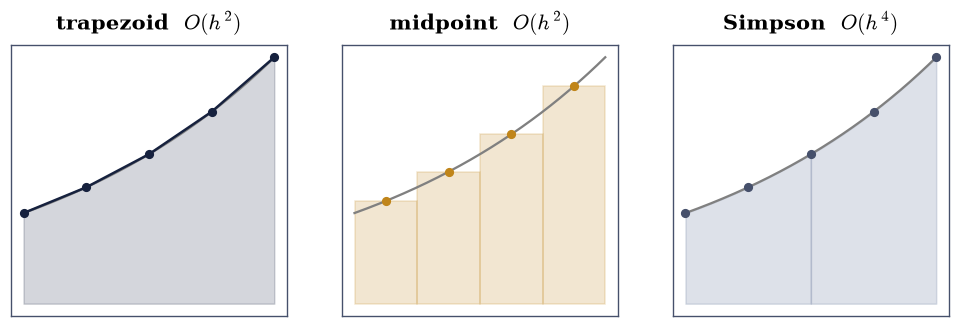
Fig. 22 How three Newton–Cotes rules sample the running integral \(\int_0^1 e^x\,dx\) over \(n=4\) panels of width \(h\): the trapezoid rule (dark) joins endpoints by straight lines, the midpoint rule (amber) uses flat panels at the centres, and Simpson’s rule (grey) fits a parabola across each pair of panels — gaining two orders of accuracy for one extra sample per pair of panels. The curve shown is \(e^x\) on \([0,1]\), the same integrand used throughout this notebook.

Solution — Exercise 1

n=  8:  trapezoid err 2.24e-03,  midpoint err 1.12e-03
n= 64:  trapezoid err 3.50e-05,  midpoint err 1.75e-05

Validation 1

✓  trapezoid rule approximates ∫₀¹eˣ (coarse)   [got 1.72052 vs expected 1.71828 (rtol=0.01, atol=1e-09)]
✓  trapezoid rule converges as panels are added   [got 1.71832 vs expected 1.71828 (rtol=0.0001, atol=1e-09)]

True

Exercise 2 — Convergence order of Newton–Cotes (worked)

The order \(p\) in error \(\approx C'n^{-p}\), Eq. 15, is what makes a rule worth using: it is minus the slope of a log–log error-vs-\(n\) plot. Trapezoid and midpoint are \(p=2\); Simpson is \(p=4\). This exercise measures those slopes directly, so it needs the fourth-order rule alongside the two second-order ones: Simpson’s rule Eq. 14 fits a parabola across each pair of panels, which is why its panel count must be even and why its weights run \(1,4,2,4,\dots,4,1\) scaled by \(h/3\).

1. Write simpson(f, a, b, n), the composite Simpson rule Eq. 14, rounding an odd \(n\) up to the next even value so the parabolas tile the interval. Write this one yourself — the implementation is the lesson.

2. For \(\int_0^1 e^x\,dx\), compute the error of each of the three rules — the trapezoid and midpoint you wrote in Exercise 1, and your simpson — over a geometric sweep of \(n\).

3. Plot the errors log–log (Fig. 23).

4. Fit the slopes with the Setup’s fit_order instrument (numpy.polyfit in log space) and compare to the theoretical orders 2, 2, 4.

measured orders:  trapezoid 2.000,  midpoint 2.000,  Simpson 3.999

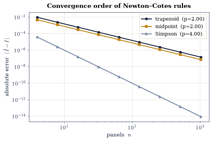
Fig. 23 Convergence of three Newton–Cotes rules on \(\int_0^1 e^x\,dx\): absolute error versus panel count \(n\) on log–log axes. The trapezoid and midpoint rules fall with slope \(-2\) (second order), Simpson with slope \(-4\) (fourth order); the midpoint error sits about a factor two below the trapezoid’s. Slopes are \(-p\) in error \(\approx C n^{-p}\) (Eq. 15).

Validation 2

✓  trapezoid is second order   [got 1.99988 vs expected 2 (rtol=1e-06, atol=0.15)]
✓  midpoint is second order   [got 1.99979 vs expected 2 (rtol=1e-06, atol=0.15)]
✓  Simpson is fourth order   [got 3.99867 vs expected 4 (rtol=1e-06, atol=0.2)]

True

Exercise 3 — Simpson’s rule and the order jump

The jump from \(O(h^2)\) to \(O(h^4)\) at Simpson’s rule Eq. 14 is the best bargain in elementary quadrature: replacing each straight-line panel by a parabola costs one extra sample per pair of panels but squares the error’s dependence on \(h\). At a fixed, modest \(n\) the difference is already dramatic.

1. For the integral \(\int_0^1 e^x\,dx\) (exact value \(e-1\)), compute the errors of the trapezoid you wrote in Exercise 1 and the simpson you wrote in Exercise 2 at the same small \(n=8\) subintervals.

2. Confirm Simpson is orders of magnitude better at identical cost.

at n=8:  trapezoid err 2.24e-03,  Simpson err 2.33e-06,  ratio 962×

Validation 3

✓  Simpson's parabolic panels gain orders over trapezoid at the same n   [Simpson 2.33e-06 vs trapezoid 2.24e-03]

True

Exercise 4 — Richardson extrapolation → Romberg

Because the trapezoid error is a clean power series in \(h^2\), two estimates at \(h\) and \(h/2\) contain enough information to cancel the leading \(O(h^2)\) term. The combination \(\big(4T(h/2)-T(h)\big)/3\), Eq. 16, is \(O(h^4)\) (Simpson’s rule in disguise) and iterating the cancellation up a triangular table is Romberg integration, which reaches very high accuracy from a handful of trapezoid evaluations.

1. For the integral \(\int_0^1 e^x\,dx\) (exact value \(e-1\)), form the Richardson combination \(\big(4T(h/2)-T(h)\big)/3\) from the estimates of your Exercise 1 trapezoid at \(n=16\) and \(n=32\), and show it is far more accurate than either input.

2. Build a small Romberg table and watch the accuracy climb column by column.

trapezoid(n=16)     err 5.59e-04
trapezoid(n=32)     err 1.40e-04
Richardson combination err 9.10e-09
Romberg corner R[4,4] err 3.31e-14

Validation 4

✓  Richardson extrapolation of trapezoid is far more accurate   [got 1.71828 vs expected 1.71828 (rtol=1e-06, atol=1e-09)]

True

Exercise 5 — Gaussian quadrature: the 2n−1 magic

Newton–Cotes fixes the nodes at equal spacing. Gaussian quadrature frees them: with \(n\) nodes and \(n\) weights chosen optimally (the nodes turn out to be the roots of the degree-\(n\) Legendre polynomial), the rule integrates every polynomial up to degree \(2n-1\) exactly (Eq. 17). So \(n=3\) points nail any quintic, and for smooth functions the error falls spectrally, faster than any power of \(n\). We map the standard interval \([-1,1]\) to \([a,b]\) by \(x\mapsto \tfrac{b-a}{2}x+\tfrac{a+b}{2}\), which also scales the sum by the Jacobian \(\tfrac{b-a}{2}\).

1. Write gauss_legendre(f, a, b, n): take the standard-interval nodes and weights from numpy.polynomial.legendre.leggauss, map the nodes onto \([a,b]\), and return the Jacobian-scaled weighted sum Eq. 17. Write this one yourself — the implementation is the lesson.

2. Integrate the polynomial \(p(x)=3x^5-2x^3+x-1\), whose exact integral over \([0,1]\) is \(-1/2\), with your 3-point Gauss rule and confirm it is exact.

3. For the smooth integral \(\int_0^1 e^x\,dx\) (exact \(e-1\)), compare its errors against those of the simpson you wrote in Exercise 2, versus the number of points (Fig. 24).

3-point Gauss on p(x)=3x⁵−2x³+x−1: -0.500000000000000  (exact -0.500000000000000)

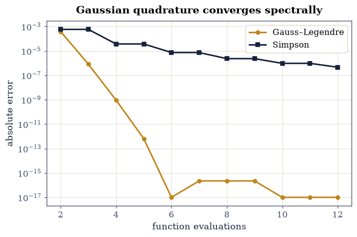
Fig. 24 Gaussian quadrature versus Simpson’s rule on the smooth integral \(\int_0^1 e^x\,dx\): absolute error against the number of function evaluations (log \(y\)). Gauss–Legendre (amber) plummets spectrally — reaching machine precision by about eight points — while Simpson (dark) falls only as a fixed power; optimising node positions as well as weights is the decisive advantage for smooth integrands.

Validation 5

✓  3-point Gauss is exact for degree ≤ 5   [got -0.5 vs expected -0.5 (rtol=1e-06, atol=1e-12)]

True

Exercise 6 — Numerical differentiation stencils

Derivatives are built the same way: combine nearby samples with weights that cancel the unwanted Taylor terms. The forward difference Eq. 18 keeps only the first term and is \(O(h)\); the central difference cancels the second-order term by symmetry and is \(O(h^2)\); the fourth-order central stencil combines four points to cancel through \(O(h^4)\). More points, higher order.

1. Write d_forward(f, x, h), d_central(f, x, h), and d_fourth(f, x, h), the three stencils of Eq. 18. Write these yourself — the implementations are the lesson.

2. Measure their orders by differentiating \(f=\sin\) at \(x=1\) (so \(f'=\cos 1\) is the exact target), fitting the error-vs-\(h\) slopes (numpy.polyfit in log space) over the truncation-dominated regime (Fig. 25).

stencil orders:  forward 1.006,  central 2.000,  4th 4.000

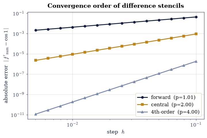
Fig. 25 Error of three finite-difference derivative stencils for \(f=\sin\) at \(x=1\) versus step \(h\), log–log, over the truncation-dominated range: the forward difference falls with slope \(1\), the central with slope \(2\), and the fourth-order central with slope \(4\) — each extra cancelled Taylor term steepens the convergence by one order (Eq. 18).

Validation 6

✓  forward difference is first order   [got 1.00588 vs expected 1 (rtol=1e-06, atol=0.15)]
✓  central difference is second order   [got 1.99988 vs expected 2 (rtol=1e-06, atol=0.15)]
✓  the 4th-order stencil is fourth order   [got 3.9997 vs expected 4 (rtol=1e-06, atol=0.2)]

True

Exercise 7 — Round-off revisited: order beats step (callback to 0.1)

§0.1 showed a single derivative’s error is U-shaped in \(h\): truncation \(\sim h^p\) falling, round-off \(\sim \varepsilon/h\) rising, with a minimum at an intermediate \(h_\star\). The order \(p\) sets how low that minimum reaches. So for a smooth function the way to a more accurate derivative is not a smaller step (round-off caps that) but a higher-order stencil, whose U bottoms out lower, and at a larger (safer) \(h\).

1. Sweep \(h\) across many decades (numpy.logspace) for the d_forward and d_central stencils you wrote in Exercise 6, and plot both U-curves on one axis (Fig. 26).

2. Confirm the central difference reaches a lower minimum error than the forward difference — and reaches it at a larger, safer step.

minimum error — forward 1.07e-10 at h=8.9e-09
minimum error — central 8.65e-13 at h=1.8e-06

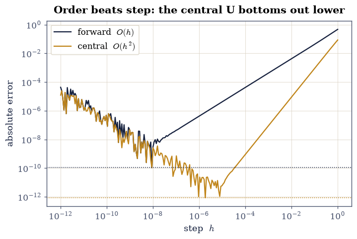
Fig. 26 The differentiation error U-curve for two stencils on \(f=\sin\) at \(x=1\): each error (forward dark, central amber) falls with truncation as \(h\) shrinks, then rises as round-off \(\sim\varepsilon/h\) takes over (the floor of §0.1). The higher-order central difference bottoms out lower and at a larger \(h\) — raising the order, not shrinking the step, is what buys accuracy for a smooth function.

Validation 7

✓  the higher-order stencil reaches a lower error floor   [central 8.65e-13 < forward 1.07e-10]

True

Exercise 8 — Adaptive quadrature in practice (synthesis)

Production integrators do not use a fixed grid: they place samples adaptively, refining only where the integrand varies, and self-estimate their error. scipy.integrate.quad (adaptive Gauss–Kronrod) is the workhorse, and it is exactly what the course leans on for the orbital and scattering integrals of §2.4–§2.5 and the descent-time integral of §2.8. On a sharply peaked integrand, a fixed grid of the same size misses the spike entirely while the adaptive rule clusters its points there and nails it.

1. Integrate the narrow Gaussian spike \(f(x)=\exp\!\big[-(x-0.5)^2/(2\cdot 0.03^2)\big]\) on \([0,1]\) with scipy.integrate.quad, against the closed form \(0.03\sqrt{2\pi}\,\operatorname{erf}\!\big(0.5/(0.03\sqrt2)\big)\approx0.0752\) (math.erf).

2. Contrast with a fixed grid of the same cost: run the trapezoid you wrote in Exercise 1 on a comparable number of evaluations, and watch it miss the spike.

adaptive quad : 0.0751988482   (≈ 231 evals, est. err 1.5e-12)
fixed trapezoid: 0.0751988482   err 0.00e+00
exact          : 0.0751988482

Validation 8

✓  adaptive quadrature matches the known integral of a sharp peak   [got 0.0751988 vs expected 0.0751988 (rtol=1e-08, atol=1e-09)]

True

Exercise 9 — Scale to order one before quad (a standing rule)

Exercise 8 handed quad a sharp peak and watched it win. That is the happy case, and it quietly hides a precondition. An adaptive routine refines where it already sees structure, so it has to find the integrand before it can refine anywhere at all, and on an infinite range it starts from a fixed transformation and a fixed handful of nodes. Nothing in that machinery knows the physical scale of the problem it was handed, and SI units issue scales like \(10^{15}\) without comment.

Blackbody radiation is the standard cautionary tale, and it is worth running rather than taking on trust. The spectral energy density of a photon gas at temperature \(T\) is Planck’s law,

(19)\[u(\omega, T) = \frac{\hbar\,\omega^3}{\pi^2 c^3}\, \frac{1}{e^{\hbar\omega/k_BT} - 1},\]

derived in §7.14 and supplied in Setup as a given integrand, its denominator evaluated with numpy.expm1 for the reason §0.1 gives. Its integral over all frequencies has a closed form, the Stefan–Boltzmann law \(u = aT^4\) with \(a = \pi^2k_B^4/15\hbar^3c^3\), so there is an exact answer to be judged against: at the Sun’s effective temperature \(T = 5772\) K it comes to \(0.8398\) J/m³.

The trouble is where the integrand lives. In SI its peak sits at \(\omega \approx 2.1\times10^{15}\) rad/s and stands some \(10^{-16}\) J·s/m³ tall, which is ordinary physics and hostile arithmetic. quad handles \((0,\infty)\) by mapping the half-line onto the unit interval with \(\omega = (1-t)/t\) and integrating the Jacobian-weighted

(20)\[g(t) = \frac{1}{t^2}\,u\!\left(\frac{1-t}{t},\,T\right), \qquad \int_0^\infty u\,d\omega = \int_0^1 g(t)\,dt\]

in its place. The peak frequency maps to \(t = 1/(1+\omega) \approx 5\times10^{-16}\), so the whole content of the integral is a needle about \(10^{-15}\) wide, standing somewhere inside a unit interval. No sampler that opens with a handful of nodes will ever tread on it.

The cure costs one substitution, made on paper before any code runs. With \(x = \hbar\omega/k_BT\),

(21)\[u = \frac{(k_BT)^4}{\pi^2\hbar^3c^3}\int_0^\infty \frac{x^3}{e^x-1}\,dx, \qquad \int_0^\infty \frac{x^3}{e^x-1}\,dx = \frac{\pi^4}{15},\]

and the integrand becomes a bump of height \(1.42\) peaking at \(x \approx 2.82\), with a tail that any cutoff past \(x \approx 60\) truncates below machine precision. Same routine, same machine, ten correct digits. Stated as a standing rule of the course, and honoured from here on: quad meets physics only after the physics has been scaled to order one. A wrong answer that arrives with no warning is the most dangerous kind.

1. Spring the trap. Integrate the dimensional Planck integrand, lambda w: u_planck(w, T_SUN), over \((0,\infty)\) with scipy.integrate.quad, wrapped in warnings.catch_warnings(record=True). Report the value returned, quad’s own error estimate, how many warnings were raised, and \(\log_{10}(aT^4/I)\): the number of orders of magnitude the silent answer is wrong by.

2. Diagnose it. Build \(g(t)\) of Eq. 20, evaluate it at the \(10^6\) uniformly spaced midpoints \((i+\tfrac12)/10^6\) of \((0,1)\), and report the largest value that grid ever sees along with its midpoint-rule estimate of the area. Both come out absurdly small: the needle is real, and it is missed.

3. Scale to order one. Write the nondimensional integrand \(x^3/(e^x-1)\) with numpy.expm1, integrate it using the same quad on \([0,60]\) (limit=200), compare against \(\pi^4/15\) from Eq. 21, and multiply by \((k_BT)^4/\pi^2\hbar^3c^3\) to recover \(aT^4\). Write this one yourself — the implementation is the lesson.

4. Put the two integrands side by side (Fig. 27): the needle in \(t\), and the order-one bump in \(x\).

dimensional quad on (0, ∞): 8.235e-38 J/m^3
  its own error estimate  : 1.6e-37   warnings raised: 0
  the true aT^4           : 0.8398 J/m^3
  → wrong by 37 orders of magnitude, silently

1,000,000 uniform samples of g(t) on (0,1):
  largest value seen      : 4.79e-21
  midpoint-rule area      : 4.87e-27   (true: 0.8398)

∫ x³/(eˣ−1) dx = 6.4939394023   (π⁴/15 = 6.4939394023)
rescaled energy density / aT^4 = 1.0000000000

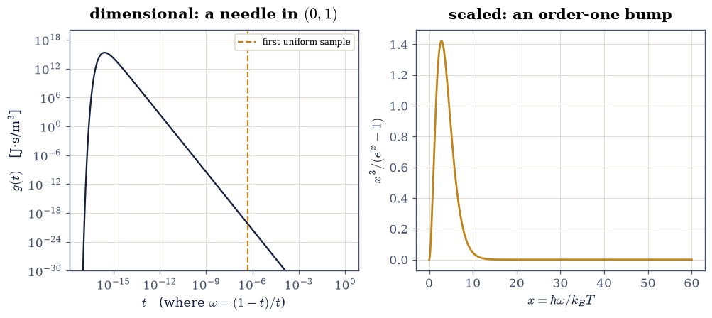
Fig. 27 The same physical integral, before and after scaling. Left: the Planck integrand after quad’s half-line map \(\omega=(1-t)/t\), \(g(t)=t^{-2}u((1-t)/t,T)\) of Eq. 20, on log–log axes at \(T=5772\) K: it peaks at \(t\approx5\times10^{-16}\) and has fallen thirty-five orders of magnitude by \(t=5\times10^{-7}\), where the first of a million uniformly spaced samples (dashed) finally looks. On a linear axis the whole feature is a needle roughly \(10^{-15}\) wide. Right: the same integral nondimensionalized by \(x=\hbar\omega/k_BT\), \(x^3/(e^x-1)\) of Eq. 21, on linear axes over the integration range \([0,60]\): a bump of height \(1.42\) at \(x\approx2.82\) that any sampler resolves.

Validation 9

✓  dimensional quad on Planck's law is wrong by >30 orders and raises no warning   [wrong by 37 orders, 0 warnings raised]
✓  a million uniform samples of the transformed integrand never touch the needle   [largest value seen 4.79e-21, against a peak of order 1e15]
✓  scaled to order one, the same quad returns π⁴/15 to ten digits   [got 6.49394 vs expected 6.49394 (rtol=1e-10, atol=1e-09)]
✓  the rescaled integral reproduces the Stefan–Boltzmann energy density aT⁴   [got 1 vs expected 1 (rtol=1e-10, atol=1e-09)]

True

Notebook summary

• Newton–Cotes quadrature with measured orders: trapezoid and midpoint second order, Simpson fourth; Richardson extrapolation building Romberg; and Gaussian quadrature exact to degree \(2n-1\).

• Finite-difference stencils (forward first order, central second, a fourth-order stencil) and the round-off-versus-truncation tradeoff (callback to §0.1); adaptive quadrature in practice.

• The standing rule that guards all of it: on Planck’s law in SI units quad returns \(8.2\times10^{-38}\) J/m³ against a true \(0.8398\) J/m³, thirty-seven orders wrong with zero warnings, because the whole integral is a \(10^{-15}\)-wide needle in the unit interval the routine actually samples. The substitution \(x=\hbar\omega/k_BT\) turns it into a bump of height \(1.42\), and the same call then returns \(\pi^4/15\) to ten digits.

Outlook

• Singular and improper integrals. Endpoint singularities and infinite ranges are tamed by variable transformations: the tanh–sinh (“double exponential”) rule is a remarkably robust default.

• Many dimensions. Tensor-product quadrature suffers the curse of dimensionality (\(n^d\) points); Monte Carlo integration trades order for dimension-independent \(O(N^{-1/2})\) error: a forward link to the statistical mechanics of Volume V.

• Spectral methods. For periodic and smooth functions a derivative stops being a difference quotient at all: transform, multiply by \(ik\), transform back, and the accuracy is exponential rather than \(O(h^p)\). The transform itself is built in §0.6, and the course puts the idea to work in the split-step propagator of §6.13, where the kinetic operator \(\hat p^2/2m\) is applied by multiplying by a phase in \(k\)-space between an FFT and its inverse — spectral differentiation, exponentiated. Clenshaw–Curtis quadrature, its quadrature counterpart, stays a named horizon.

• Automatic differentiation. The exact alternative to finite differences: derivatives to machine precision with no step to tune, and the engine behind modern machine learning and gradient-based physics.

References

[Hig02]

Nicholas J. Higham. Accuracy and Stability of Numerical Algorithms. Society for Industrial and Applied Mathematics (SIAM), 2 edition, 2002.

[PTVF07]

William H. Press, Saul A. Teukolsky, William T. Vetterling, and Brian P. Flannery. Numerical Recipes: The Art of Scientific Computing. Cambridge University Press, 3 edition, 2007.

Take this notebook with you

Use the download button (↓) in the toolbar above to save this notebook and run it yourself. The published notebooks ship without worked solutions; if you would like the reference solutions — to teach from or to check your own work — get in touch: hello@ramador.me.