


5.7 Thermodynamic Potentials, Legendre Transforms, and the Maxwell Relations#
Notebook overview#
§5.6 gave us the fundamental relation \(dU=T\,dS-P\,dV+\mu\,dN\), and with it the entropy \(S(E,V,N)\) and energy \(U(S,V,N)\) of a gas. But there is a quiet practical problem with those two functions: nobody controls a system’s entropy or energy. A laboratory thermostat fixes the temperature \(T\), not the entropy; a piston fixes the pressure \(P\), not the volume; a particle reservoir fixes the chemical potential \(\mu\), not the number. The natural variables of \(S\) and \(U\) are the wrong ones. This notebook builds the functions whose natural variables are the ones we hold fixed — the thermodynamic potentials \(F(T,V,N)\), \(H(S,P,N)\), \(G(T,P,N)\), \(\Phi(T,V,\mu)\) — and the single mathematical machine that generates them all: the Legendre transform.
That machine is not new. It is exactly the operation that took the Lagrangian to the Hamiltonian in Volume II, \(H(q,p)=\max_{\dot q}[p\dot q-L(q,\dot q)]\), trading the velocity \(\dot q\) for its conjugate slope \(p=\partial L/\partial\dot q\). Here it trades entropy for temperature, \(F=U-TS\), and volume for pressure, and number for chemical potential. We make the unity literal: we will write one numerical convex-conjugate routine and run it on both the mechanical \(L=\tfrac12 m\dot q^2\to H=p^2/2m\) and the thermodynamic \(U(S)\to F(T)\) — the same code, two domains. This structural unity across the whole course is the heart of the notebook.
From the potentials, three things follow, and we develop each in full. Their first derivatives return the conjugate variables (\(-S=(\partial F/\partial T)_V\), and so on). Their mixed second partials are equal regardless of order — Clairaut’s theorem — and that single fact, applied to the four potentials, gives the four Maxwell relations, a web of non-obvious identities that trade a hard-to-measure quantity for an easy one. (The Maxwell relations get the room the subject deserves: all four, each derived as a mixed partial, each verified, each with its physical use.) Their pure second derivatives are the response functions — the heat capacity, the compressibility — whose positivity is nothing other than thermodynamic stability, the convexity of the potentials. And each potential is minimized at equilibrium, the thermodynamic face of the entropy maximization of §5.4 — the principle that explains why things melt, mix, and order.
This notebook runs long by design; the structure it builds is the working architecture of thermodynamics, and §5.8 will ground it statistically when the canonical ensemble delivers \(F=-kT\ln Z\) directly. We work with the monatomic ideal gas in units \(N=k=1\), handling the entropy constant so that \(S(U)\) and \(U(S)\) are exact inverses — the one place a numerical Legendre transform silently goes wrong, flagged where it matters.
How to read the checks. Each exercise closes with a
validatecall against an independent fact: the conjugate pairs assembling to an energy; the numerical Legendre transform reproducing analytic conjugates; the same routine giving \(H=p^2/2m\) and \(F=-U^*(T)\) (the sign flip); the potential identities; each of the four Maxwell relations as an equality of mixed partials; the free energy minimized at \(m=\tanh(h/kT)\); the response functions \(C_V=\tfrac32\), \(\kappa_T=1/P\) positive; and Joule’s \((\partial U/\partial V)_T=0\). A ✓ is strong evidence; a ✗ is a prompt to locate the discrepancy.Scope. The architecture of equilibrium thermodynamics from the fundamental relation. The statistical grounding \(F=-kT\ln Z\) and the response-functions-as-fluctuations are §5.8; the grand potential and its ensemble later in the volume; criticality (where stability breaks) is §5.10. See Callen, Thermodynamics; Schroeder; Kardar; and Volume II (the Legendre transform \(L\to H\)), §5.4 (entropy maximization, the paramagnet), §5.6 (the fundamental relation).
Theory in brief#
The problem: the wrong natural variables#
The fundamental relation makes \(U\) a function of \((S,V,N)\) and \(S\) a function of \((E,V,N)\). But a laboratory does not control \(S\) or \(E\) — it controls \(T\), \(P\), \(\mu\),
We need potentials whose natural variables are the controlled ones. The Legendre transform builds them.
The Legendre transform#
For a convex \(f(x)\), the Legendre (convex-conjugate) transform is
a function of the slope \(p=f'(x)\) rather than of \(x\): it encodes \(f\) by its family of tangent lines (slope \(p\), intercept \(-f^*(p)\)) instead of by its points, invertibly (\(f^{**}=f\)). This is exactly Volume II’s \(H(q,p)=\max_{\dot q}[p\dot q-L]\) with \(p=\partial L/\partial\dot q\). The transform swaps a variable for its conjugate slope.
The four thermodynamic potentials#
Legendre-transforming \(U(S,V,N)\) in each conjugate pair gives
An honest subtlety of sign: thermodynamics minimizes, so the free energy is the negative of the mathematician’s convex conjugate, \(F=-U^*(T)=\min_S[U-TS]\), not \(\max\). We verify this numerically and flag it — it is exactly where sign errors hide.
The Maxwell relations#
For a \(C^2\) potential the mixed second partials commute (Clairaut’s theorem — a calculus fact, stated not proved). Applied to each potential, this gives one identity apiece,
from \(U,H,F,G\) respectively. Their power: they trade a hard-to-measure quantity (an entropy change) for an easy one (a pressure or volume response).
The variational principle, and stability#
Each potential is minimized at equilibrium under its natural constraints — \(F\) at fixed \((T,V)\), \(G\) at fixed \((T,P)\) Eq. 613 — the Legendre image of “\(S\) maximized at fixed \(E\)” (§5.4). \(F=U-TS\) is the competition between energy minimization and entropy maximization, the central idea of why matter melts, mixes, and orders. Finally, the transform flips convexity (\(U\) convex in \(S\Rightarrow F\) concave in \(T\)), and the response functions are the pure second derivatives,
whose positivity (\(C_V>0\), \(\kappa_T>0\)) is thermodynamic stability. These equal the fluctuations of §5.8 (\(\operatorname{Var}(E)=kT^2C_V\)), and can diverge at a critical point (§5.10).
Setup#
Data and instruments only: the series palette, and the monatomic ideal gas itself — its energy
\(U(S,V)\) together with the closed forms of \(F\), \(S\), \(P\), \(V\) and \(T\) in each pair of natural
variables, every one of them a displayed equation transcribed rather than machinery anyone
builds — plus the central-difference derivative stencil of
§0.3, restated here in a
select-one-argument form so it can take the thermodynamic partials and, applied twice, the
mixed partials of the Maxwell relations. The notebook’s own machine is not here: you write
the numerical Legendre transform convex_conjugate in Exercise 2, and every transform from
Exercise 3 onward runs through it. No randomness appears anywhere in this notebook.
The Setup below holds this notebook’s data and instruments — nothing you are asked to build. It is collapsed so the building stays yours; expand it whenever you want the details.
Exercise 1 — The wrong natural variables (worked)#
We begin with the motivation, because it is the reason the rest of the notebook exists. The fundamental relation \(dU=T\,dS-P\,dV+\mu\,dN\) presents the energy as \(U(S,V,N)\) and the entropy as \(S(E,V,N)\). Mathematically those are complete descriptions. Experimentally they are awkward, because their independent variables — entropy, energy, particle number, volume — are mostly not what an apparatus holds fixed (Fig. 436). A thermostat sets the temperature; a piston open to the atmosphere sets the pressure; a membrane to a reservoir sets the chemical potential. Notice the structure: the relation pairs each “extensive” variable we struggle to control (\(S\), \(V\), \(N\)) with an “intensive” conjugate slope we can control (\(T\), \(-P\), \(\mu\)), and each pair multiplies to an energy (\(TS\), \(PV\), \(\mu N\)). The plan of the whole subject is to trade each inconvenient variable for its convenient conjugate — and the Euler relation \(U=TS-PV+\mu N\) is the promise that nothing is lost in the trade: the conjugate products reassemble the energy exactly.
Testing that promise honestly takes one precaution. Setting \(\mu\equiv G\) would rebuild \(U\) identically and so test nothing, so the chemical potential has to arrive by an independent route: \(\mu=-T(\partial S/\partial N)_{U,V}\) evaluated on the extensive entropy \(S(U,V,N)=N[\ln(V/N)+\tfrac32\ln(U/N)]\), the route of §5.6. That form is first-order homogeneous in \((U,V,N)\) and reduces to our \(S(U,V)\) at \(N=1\) with the same constant \(s_0=0\), so the Euler relation then genuinely tests the extensivity of \(S\) rather than restating the definition of \(G\). We work at the reference state \(T=V=1\), where the caloric equation of state gives \(U=\tfrac32\).
Part a) Compute \(U\), \(S\), \(P\) and \(G\) at the reference state, and obtain \(\mu\) independently as \(-T\,\partial S/\partial N\) by a symmetric finite difference of \(S(U,V,N)\) in the particle number at fixed \(U\) and \(V\).
Part b) Confirm the Euler relation \(U=TS-PV+\mu N\), and that the independently obtained \(\mu\) equals \(G/N\) — the Gibbs potential is the chemical potential per particle.
Part c) Collect each potential beside its natural variables and the Legendre trade that builds it from \(U\), as one table (Fig. 436).
ideal gas at T=1.0, V=1.0:  U=1.5000, S=0.6082, P=1.0000
μ = −T ∂S/∂N (independent finite difference) = 1.8918   vs  G/N = 1.8918
conjugate-pair products: TS=0.6082, PV=1.0000, μN=1.8918  (each an energy)
Euler relation TS − PV + μN = 1.5000   vs   U = 1.5000
Validation 1#
✓  Euler: U = TS − PV + μN, with μ from the independent −T ∂S/∂N route — extensivity, tested   [got 1.5 vs expected 1.5 (rtol=1e-06, atol=1e-09)]
✓  the independent μ equals G/N — the Gibbs potential is the chemical potential per particle   [got 1.8918 vs expected 1.8918 (rtol=1e-06, atol=1e-09)]
True
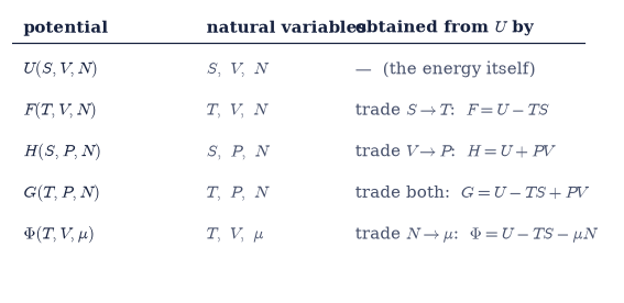
Fig. 436 Why we need new potentials: the conjugate pairs and what each potential holds fixed. The fundamental relation pairs each extensive variable (\(S\), \(V\), \(N\)) with an intensive conjugate slope (\(T\), \(-P\), \(\mu\)); each pair multiplies to an energy. A laboratory controls the intensive members (temperature, pressure, chemical potential), not the extensive ones — so for each set of controlled variables there is a potential (\(U\), \(F\), \(H\), \(G\), \(\Phi\)) whose natural variables are exactly those. The Legendre transform is the machine that swaps an extensive variable for its conjugate slope, building each potential from \(U\).#
Exercise 2 — The Legendre transform, geometrically (worked)#
Before applying it, we build the Legendre transform from scratch and see what it does. The definition \(f^*(p)=\max_x[p\,x-f(x)]\) Eq. 418 looks abstract, but it has a vivid geometric meaning (Fig. 437). For a fixed slope \(p\), the line \(y=p\,x\) sits above the convex curve \(f\) in some places and below in others; \(p\,x-f(x)\) is the vertical gap, and its maximum over \(x\) occurs where the line is parallel to the curve, i.e. where \(f'(x)=p\). At that point the tangent line of slope \(p\) touches the curve, and its \(y\)-intercept is exactly \(-f^*(p)\). So the transform re-describes the curve by its family of tangent lines — slope and intercept — instead of by its points. No information is lost: for a convex function the transform is its own inverse, \(f^{**}=f\). The whole of the next several exercises is this one operation, applied where the “curve” is a Lagrangian or an energy.
The specimen to certify against is the parabola \(f(x)=x^2\), whose conjugate is exactly \(f^*(p)=p^2/4\): the tangent of slope \(p\) touches at \(x=p/2\), where \(px-x^2\) takes the value \(p^2/4\). Transforming \(p^2/4\) in turn must return the parabola, which is involutivity made concrete.
Part a) Write convex_conjugate(f, xgrid, p), the numerical Legendre transform
\(f^*(p)=\max_x[p\,x-f(x)]\) Eq. 418: for each requested slope, form the gap
\(p\,x-f(x)\) on the grid xgrid and take its largest value over \(x\). Broadcast the slopes
against the grid — slopes down one axis, grid points along the other — so that a whole family
of conjugates comes out of a single numpy.max. Its accuracy is set by the grid spacing and by
the grid being wide enough to contain the maximizer \(x^*=f'^{-1}(p)\), so both are the caller’s
responsibility. Write this one yourself — the implementation is the lesson, and every
Legendre transform in this notebook, mechanical and thermodynamic, runs through it.
Part b) Certify it against the closed form at the slopes \(p=0.5,\,1,\,2,\,3\), and check involutivity by transforming \(p^2/4\) back and recovering \(f(2)=4\).
Part c) See the geometry move: roll a tangent line of slope \(p\) along the curve and watch its intercept trace out \(-f^*(p)\) (Fig. 437).
f(x) = x²   →   f*(p) = p²/4
  slopes p        = [0.5 1.  2.  3. ]
  numeric  f*(p)  = [0.0625 0.25   1.     2.25  ]
  analytic p²/4   = [0.0625 0.25   1.     2.25  ]
  involutive f**=f at x=2: 4.0000 vs f(2)=4.0000
Validation 2#
✓ the numerical Legendre transform reproduces the analytic convex conjugate (f=x² → f*=p²/4) [max|Δ| = 1e-06 (rtol=0.001, atol=1e-09)]
True
Fig. 437 The Legendre transform as a rolling tangent line (animated). The convex curve \(f(x)=x^2\) (dark) is re-encoded by its tangent lines: for each slope \(p\) the tangent (amber) touches where \(f'(x)=p\), and its \(y\)-intercept is \(-f^*(p)\). As the slope rolls, the intercept traces the conjugate \(-f^*(p)=-p^2/4\) (the lower curve). Describing the curve by its tangents (slope, intercept) instead of its points is the whole transform — invertible, information-preserving, and the same operation that will trade entropy for temperature.#
Exercise 3 — The Legendre transform is one operation: Volume II meets thermodynamics (worked)#
This is the heart of the notebook, and the moment the course’s structure shows itself. The
Legendre transform we just built is the same operation that took the Lagrangian to the
Hamiltonian in Volume II. There, \(H(q,p)=\max_{\dot q}[p\dot q-L(q,\dot q)]\) traded the velocity
\(\dot q\) for the momentum \(p=\partial L/\partial\dot q\). Here, trading the entropy \(S\) for the
temperature \(T\) turns the energy \(U(S,V)\) into the Helmholtz free energy. To prove the unity is
real and not a slogan, one routine has to serve both: the mechanical \(L=\tfrac12 m\dot q^2\),
whose transform must give \(H=p^2/2m\), and the thermodynamic \(U(S,V)\) at fixed \(V\), whose
transform must give the free energy already available in closed form as F_TV. One catch, and
it is the honest subtlety of the whole subject: thermodynamics minimizes the potential, so the
free energy is the negative of the mathematician’s convex conjugate,
\(F=-U^*(T)=\min_S[U-TS]\) rather than \(\max\). It is exactly where errors hide, so the sign flip
gets verified rather than asserted.
Part a) With the convex_conjugate you wrote in Exercise 2, transform the mechanical
Lagrangian \(L=\tfrac12 m\dot q^2\) at \(m=2\) and confirm it returns \(H=p^2/2m\) at the momenta
\(p=1,\,2,\,3\) (Volume II).
Part b) Run that same routine on the ideal-gas energy \(U(S,V)\) at fixed \(V\) and recover the
free energy as \(F=-U^*(T)\) at \(T=0.8,\,1,\,1.5\), checked against the closed-form F_TV. The
entropy grid has to be wide enough to hold the maximizer at every temperature asked for.
(a) mechanics:  L = ½mq̇²  →  H(p)
    numeric H = [0.25 1.   2.25]   vs   p²/2m = [0.25 1.   2.25]
(b) thermodynamics:  U(S,V)  →  F = −U*(T)  (minimize, not maximize)
    F from Legendre = [0.98121 0.8918  0.42541]
    F closed form   = [0.98121 0.8918  0.42541]
Validation 3#
✓  the same Legendre routine sends L = ½mq̇² to H = p²/2m (Volume II)   [max|Δ| = 1.77778e-06 (rtol=0.001, atol=1e-09)]
✓  and sends U(S) to the free energy F = −U*(T) — the thermodynamic sign flip   [max|Δ| = 6.13574e-09 (rtol=0.002, atol=1e-09)]
True
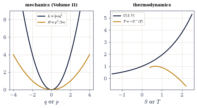
Fig. 438 One operation, two domains. Left: the Legendre transform of the mechanical Lagrangian \(L=\tfrac12 m\dot q^2\) (dark) is the Hamiltonian \(H=p^2/2m\) (amber) — Volume II, run through our numerical convex_conjugate. Right: the same routine on the ideal-gas energy \(U(S,V)\) at fixed \(V\) (dark) gives the Helmholtz free energy \(F=-U^*(T)\) (amber), with the thermodynamic sign flip (minimize, not maximize). The operation that traded velocity for momentum in mechanics trades entropy for temperature in thermodynamics — identical mathematics, and the structural keystone of the course.#
Exercise 4 — The four potentials and their differentials (worked)#
With the machine established, we lay out its four products and check that they behave. From \(U(S,V,N)\) we built \(F=U-TS\), \(H=U+PV\), \(G=U-TS+PV\), and \(\Phi=U-TS-\mu N\) Eq. 419, and each came with a differential whose structure tells us its natural variables: \(dF=-S\,dT- P\,dV+\mu\,dN\) has natural variables \((T,V,N)\), and so on. Two consistency checks confirm we have them right. First, the potentials satisfy the obvious algebraic identities among themselves, e.g. \(G=F+PV=H-TS\). Second, and more usefully, each potential’s first derivatives return the conjugate variables: from \(dF=-S\,dT-P\,dV\) we must have \(-S=(\partial F/\partial T)_V\) and \(-P=(\partial F/\partial V)_T\). That second check is the working definition of a potential — it is how one extracts \(S\) and \(P\) from \(F\). Reaching \(G\) as a function of \((T,P)\) takes one small manoeuvre: the Setup gives \(F\) in \((T,V)\), so \(G(T,P)=F(T,V)+PV\) evaluated along \(V=T/P\).
Part a) At the reference state of Exercise 1, compute \(F\), \(H\) and \(G\), and confirm the algebraic identity \(G=F+PV\) against \(G\) assembled directly as \(U-TS+PV\).
Part b) Confirm the first-derivative identities \(-S=(\partial F/\partial T)_V\) and
\(V=(\partial G/\partial P)_T\) by finite differences with the Setup’s partial stencil.
F=0.8918, H=2.5000, G=1.8918
identity  G = F + PV:  1.8918  vs  1.8918
first derivative  −(∂F/∂T)_V = 0.6082  vs  S = 0.6082
first derivative   (∂G/∂P)_T = 1.0000  vs  V = 1.0000
Validation 4#
✓ the potentials satisfy G = F + PV and their first derivatives recover the conjugate variables (−∂F/∂T = S, ∂G/∂P = V) [max|Δ| = 3.98579e-11 (rtol=0.001, atol=1e-09)]
True
Exercise 5 — Maxwell relation I, from \(F(T,V)\): the workhorse (worked)#
Now the part the structure was built for, and the part we develop most carefully. Every potential is a smooth function of two (or more) variables, and for any such \(C^2\) function the mixed second partial derivatives are equal regardless of the order of differentiation — Clairaut’s theorem. We take that as the calculus fact it is and do not prove it; what matters is what it says about thermodynamics. Take \(F(T,V)\) with \(dF=-S\,dT-P\,dV\), so that \((\partial F/\partial T)_V=-S\) and \((\partial F/\partial V)_T=-P\). Differentiate the first by \(V\) and the second by \(T\): both equal \(\partial^2 F/\partial T\,\partial V\), so \(-(\partial S/\partial V)_T=-(\partial P/\partial T)_V\), i.e. $\(\left(\frac{\partial S}{\partial V}\right)_T=\left(\frac{\partial P}{\partial T}\right)_V\)\( {eq}`eq-maxwell-relations`. This is the workhorse Maxwell relation, and its power is practical: the left side is an *entropy* change with volume — almost impossible to measure directly — while the right side is how pressure responds to temperature at fixed volume, an easy gauge reading. The relation lets one stand in for the other. For the ideal gas both sides equal \)N/V\(, which is \)1$ at our reference state.
Part a) Evaluate the two sides separately with the Setup’s partial stencil — the entropy
slope from \(S(T,V)\), the pressure slope from \(P(T,V)\) — at the reference state.
Part b) Confirm that they agree, and that both land on \(N/V\): an entropy-volume slope nobody can measure, read off a pressure gauge instead.
Maxwell relation from F(T,V):   (∂S/∂V)_T  =  (∂P/∂T)_V
  (∂S/∂V)_T = 1.000000
  (∂P/∂T)_V = 1.000000    (both = N/V = 1.000000)
  use: an unmeasurable entropy-volume slope, read off from a pressure gauge
Validation 5#
✓ Maxwell relation from F: (∂S/∂V)_T = (∂P/∂T)_V [got 1 vs expected 1 (rtol=0.001, atol=1e-09)]
True
Exercise 6 — Maxwell relation II, from \(G(T,P)\) (worked)#
The same move on the next potential gives the next relation. Take \(G(T,P)\) with \(dG=-S\,dT+V\,dP\), so \((\partial G/\partial T)_P=-S\) and \((\partial G/\partial P)_T=V\). Equating the mixed partial \(\partial^2 G/\partial T\,\partial P\) both ways gives \(-(\partial S/\partial P)_T=(\partial V/\partial T)_P\), that is $\(\left(\frac{\partial S}{\partial P}\right)_T=-\left(\frac{\partial V}{\partial T}\right)_P\)\( {eq}`eq-maxwell-relations`. Note the **sign**: it is set entirely by the \)+V,dP\( in \)dG\( (versus the \)-P,dV\( in \)dF\(), and getting it from the differential rather than from memory is the whole point of the method. Physically this trades the entropy's response to pressure (hard) for the thermal expansion (easy — watch the volume grow as you warm it). For the ideal gas both sides are \)-N/P\(. The natural variables here are \)(T,P)\(, so the two slopes come from \)S(T,P)\( and \)V(T,P)$.
Part a) Evaluate \((\partial S/\partial P)_T\) and \((\partial V/\partial T)_P\) with the
partial stencil at the reference state.
Part b) Confirm \((\partial S/\partial P)_T=-(\partial V/\partial T)_P\), both equal to \(-N/P\), and satisfy yourself that the minus sign was read off the \(+V\,dP\) in \(dG\) rather than recalled.
Maxwell relation from G(T,P):   (∂S/∂P)_T  =  −(∂V/∂T)_P
  (∂S/∂P)_T  = -1.000000
  −(∂V/∂T)_P = -1.000000    (both = −N/P = -1.000000)
  the minus sign is set by the +V dP in dG — read off the differential, never memorized
Validation 6#
✓ Maxwell relation from G: (∂S/∂P)_T = −(∂V/∂T)_P [got -1 vs expected -1 (rtol=0.001, atol=1e-09)]
True
Exercise 7 — Maxwell relations III and IV, from \(U(S,V)\) and \(H(S,P)\): the adiabatic pair (worked)#
The remaining two relations come from the potentials whose natural variables include the entropy, \(U(S,V)\) and \(H(S,P)\), so they hold \(S\) fixed — they are the adiabatic pair, statements about processes at constant entropy. From \(dU=T\,dS-P\,dV\), the mixed partial \(\partial^2 U/\partial S\,\partial V\) gives \((\partial T/\partial V)_S=-(\partial P/\partial S)_V\); from \(dH=T\,dS+V\,dP\), \(\partial^2 H/\partial S\,\partial P\) gives \((\partial T/\partial P)_S=(\partial V/\partial S)_P\) Eq. 420. Because these hold the entropy fixed, we verify them along the ideal-gas adiabat (where \(TV^{2/3}\) and \(TP^{-2/5}\) are constant), differentiating the constant-entropy functions \(T(S,V)\), \(P(S,V)\), \(T(S,P)\), \(V(S,P)\) that the Setup supplies. That completes the set: four potentials, four Maxwell relations, each the equality of one potential’s mixed second partials, each with its own sign and its own use.
Part a) Take the four constant-entropy slopes at the reference state with the partial
stencil: \((\partial T/\partial V)_S\) and \((\partial P/\partial S)_V\) from \(T(S,V)\) and \(P(S,V)\),
then \((\partial T/\partial P)_S\) and \((\partial V/\partial S)_P\) from \(T(S,P)\) and \(V(S,P)\).
Part b) Confirm both adiabatic relations: \((\partial T/\partial V)_S=-(\partial P/\partial S)_V\) from \(U\), and \((\partial T/\partial P)_S=(\partial V/\partial S)_P\) from \(H\).
Part c) Assemble all four relations into one table (Fig. 439), each shown beside the two numbers this notebook actually measured for it.
Maxwell from U(S,V):  (∂T/∂V)_S = −(∂P/∂S)_V
   -0.666667  =  -0.666667
Maxwell from H(S,P):  (∂T/∂P)_S =  (∂V/∂S)_P
   0.400000  =  0.400000

the four Maxwell relations (one per potential):
  U(S,V): (∂T/∂V)_S = −(∂P/∂S)_V    H(S,P): (∂T/∂P)_S = (∂V/∂S)_P
  F(T,V): (∂S/∂V)_T =  (∂P/∂T)_V    G(T,P): (∂S/∂P)_T = −(∂V/∂T)_P
Validation 7#
✓ Maxwell relations from U and H (the adiabatic pair): (∂T/∂V)_S = −(∂P/∂S)_V and (∂T/∂P)_S = (∂V/∂S)_P [max|Δ| = 4.44089e-11 (rtol=0.001, atol=1e-09)]
True
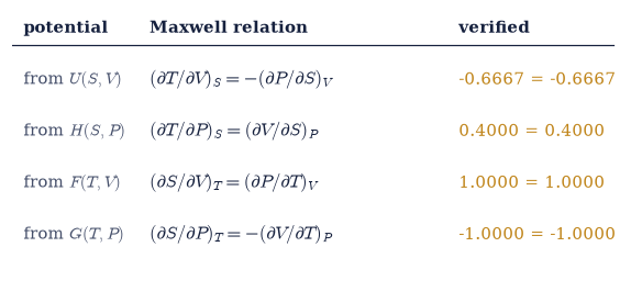
Fig. 439 The four Maxwell relations, one per potential. Each is the statement that a potential’s mixed second partials commute (Clairaut): differentiating \(-S=(\partial F/\partial T)_V\) by \(V\) equals differentiating \(-P=(\partial F/\partial V)_T\) by \(T\), and so on. The sign of each relation is read directly off the signs in that potential’s differential. The adiabatic pair (from \(U\) and \(H\)) holds entropy fixed; the isothermal pair (from \(F\) and \(G\)) holds temperature fixed. Their use is always the same: replace a quantity that is hard to measure (an entropy change) with one that is easy (a mechanical or thermal response). All four are verified numerically for the ideal gas in this notebook.#
Exercise 8 — The variational principle: free energy minimized (worked)#
We now reach the physical payoff that makes the free energy the most-used quantity in physical chemistry and condensed matter. The entropy-maximization principle of §5.4 says an isolated system at fixed energy drifts to maximum entropy. Legendre-transform that statement — trade fixed energy for fixed temperature — and it becomes: a system at fixed \((T,V)\) drifts to minimum Helmholtz free energy Eq. 613. The reason \(F=U-TS\) is so powerful is written in its two terms: minimizing \(F\) balances lowering the energy \(U\) against raising the entropy \(S\), weighted by temperature. At low \(T\) energy wins (systems order); at high \(T\) entropy wins (systems disorder). That single competition is why ice melts, why oil and water unmix, why magnets align. We demonstrate it on the paramagnet of §5.4: write its free energy per spin \(F(m)=-h\,m-T\,s(m)\) with the spin entropy \(s(m)\), minimize over the magnetization \(m\), and recover \(m=\tanh(h/kT)\) (Fig. 440). Adding an interaction — an internal field proportional to \(m\) — will make this same minimization produce spontaneous magnetization with no external field at all, the story of §5.10. The spin entropy per spin is the binary form \(s(m)=-[\tfrac{1+m}{2}\ln\tfrac{1+m}{2}+\tfrac{1-m}{2}\ln\tfrac{1-m}{2}]\), singular at the saturated ends \(m=\pm1\), so the search grid must stop just short of them.
Part a) Write down the spin entropy \(s(m)\) and the free energy per spin
\(F(m)=-h\,m-T\,s(m)\), and minimize \(F\) over \(m\) on a dense grid (numpy.argmin) at the three
combinations \((h,T)=(0.5,1),\,(1,1),\,(0.3,0.5)\).
Part b) Confirm that each minimizer is the paramagnet’s \(m=\tanh(h/kT)\) — equilibrium minimizes the free energy, and the cold system magnetizes more because \(-hm\) then outweighs \(-Ts(m)\) (Fig. 440).
minimize F(m) = −hm − T s(m) over the magnetization m:
  h=0.5, T=1.0:  argmin_m F = 0.4621   vs   tanh(h/kT) = 0.4621
  h=1.0, T=1.0:  argmin_m F = 0.7616   vs   tanh(h/kT) = 0.7616
  h=0.3, T=0.5:  argmin_m F = 0.5370   vs   tanh(h/kT) = 0.5370
Validation 8#
✓ minimizing F(m) over the magnetization gives m = tanh(h/kT) — equilibrium minimizes the free energy [got 0.462104 vs expected 0.462117 (rtol=1e-06, atol=0.002)]
True
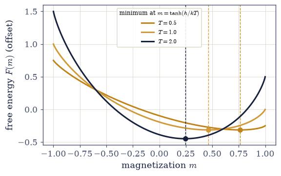
Fig. 440 Equilibrium minimizes the free energy. The paramagnet free energy per spin \(F(m)=-hm-Ts(m)\) against magnetization \(m\), at field \(h=0.5\) for three temperatures. Each curve’s minimum (dot) sits at \(m=\tanh(h/kT)\) (dashed verticals): colder systems magnetize more, because the energy term \(-hm\) wins over the entropy term \(-Ts(m)\) when \(T\) is small. This is the energy-versus-entropy competition that \(F=U-TS\) encodes — and adding an internal field \(\propto m\) turns the same minimization into spontaneous order with no external field, the phase transition of §5.10.#
Exercise 9 — Convexity, response functions, and stability (worked)#
The second derivatives of the potentials carry the last piece of the structure, and it ties
geometry to measurable physics. The Legendre transform flips convexity: \(U\) is convex in \(S\)
(its graph curves upward), and its conjugate \(F\) is concave in \(T\) (curves downward) — we can see
it directly in the curvatures. Those curvatures are the response functions. The heat capacity
is \(C_V=-T(\partial^2 F/\partial T^2)_V\), and the isothermal compressibility is \(\kappa_T=
-\tfrac1V(\partial V/\partial P)_T\) Eq. 421. Here is the deep point: their positivity
is thermodynamic stability. \(C_V>0\) means adding heat raises the temperature (a system that
cooled as you heated it would run away); \(\kappa_T>0\) means squeezing raises the pressure. Each is
exactly the statement that the relevant potential is convex/concave the right way — stability is
convexity. For the ideal gas \(C_V=\tfrac32\) and \(\kappa_T=1/P\), both safely positive. These same
response functions will reappear in §5.8 as the fluctuations of the canonical ensemble
(\(\operatorname{Var}(E)=kT^2C_V\)), and at a critical point (§5.10) they diverge as stability fails.
A second derivative differences twice, so its round-off floor sits far higher than a first
derivative’s: a coarser step than the partial default is the right choice here.
Part a) Confirm the convexity flip with three-point second differences: \(U''(S)>0\) at fixed \(V\), and \(F''(T)<0\) at fixed \(V\).
Part b) Compute the two response functions — \(C_V=-T(\partial^2 F/\partial T^2)_V\) from that
same curvature, and \(\kappa_T=-\tfrac1V(\partial V/\partial P)_T\) from the partial stencil on
\(V(T,P)\) — and confirm both are positive with \(C_V=\tfrac32\) and \(\kappa_T=1/P\).
convexity flip:  U''(S) = +0.6667 (>0, convex)   F''(T) = -1.5000 (<0, concave)
heat capacity         C_V = −T ∂²F/∂T² = 1.5000   (expect 3/2)
isothermal compress.  κ_T = −(1/V)(∂V/∂P)_T = 1.0000   (expect 1/P = 1.0000)
their positivity IS thermodynamic stability (= the convexity of the potentials)
Validation 9#
✓  the Legendre transform flips convexity: U convex in S, F concave in T
✓  the response functions C_V = −T∂²F/∂T² and κ_T are second derivatives of the potentials; their positivity is stability   [max|Δ| = 1.98602e-09 (rtol=0.01, atol=1e-09)]
True
Exercise 10 — A thermodynamic identity by a Maxwell relation (student)#
To show the Maxwell relations are tools and not ornaments, we use one to prove a result that is far from obvious by inspection: that the internal energy of an ideal gas does not depend on its volume at fixed temperature, \((\partial U/\partial V)_T=0\). This is Joule’s experimental finding (a gas expanding into vacuum at fixed temperature neither heats nor cools), and it follows in two lines. Starting from \(dU=T\,dS-P\,dV\) and dividing by \(dV\) at fixed \(T\), \((\partial U/\partial V)_T=T(\partial S/\partial V)_T-P\). Now apply the \(F\)-Maxwell relation of Exercise 5, \((\partial S/\partial V)_T=(\partial P/\partial T)_V\), to convert the unmeasurable entropy term into a pressure response: \((\partial U/\partial V)_T=T(\partial P/\partial T)_V-P\). For the ideal gas \(P=NkT/V\) gives \(T(\partial P/\partial T)_V=T\cdot N k/V=P\), so the two terms cancel exactly and \((\partial U/\partial V)_T=0\). The energy depends only on temperature — equipartition again, now derived from a Maxwell relation.
Part a) Evaluate the right-hand side \(T(\partial P/\partial T)_V-P\) for the ideal gas at the
reference state, taking the pressure slope with the partial stencil on \(P(T,V)\).
Part b) Confirm that the two terms cancel, so \((\partial U/\partial V)_T=0\) — Joule’s result, and with it the fact that an ideal gas’s internal energy depends on temperature alone.
Joule:  (∂U/∂V)_T = T(∂P/∂T)_V − P   [using the F-Maxwell relation (∂S/∂V)_T = (∂P/∂T)_V]
  = T·(N/V) − P = 1.0000 − 1.0000 = 1.00e-12
  the internal energy of an ideal gas depends only on temperature (equipartition, derived)
Validation 10#
✓ for an ideal gas (∂U/∂V)_T = 0 (Joule), shown via the F-Maxwell relation [got 1.00009e-12 vs expected 0 (rtol=1e-06, atol=0.001)]
True
Exercise 11 — The architecture of thermodynamics (synthesis)#
Step back and see the building whole. We started from a single differential, the fundamental relation \(dU=T\,dS-P\,dV+\mu\,dN\) of §5.6, and one operation, the Legendre transform of Volume II. From them the entire structure of equilibrium thermodynamics assembled itself. The transform generated the four potentials, each tuned to the variables a laboratory actually controls. Their first derivatives return the conjugate variables. Their mixed second partials, equal by Clairaut, are the four Maxwell relations — the web of identities that trade hard measurements for easy ones, which we built one by one. Their pure second derivatives are the response functions, whose positivity is stability, the convexity of the potentials made physical. And each potential is minimized at equilibrium, the Legendre image of entropy maximization, the principle behind why matter melts, mixes, and orders. Thermodynamics is not a pile of formulas to memorize; it is one architecture — one transform, four potentials, four relations, one variational principle — hanging from \(dU=T\,dS-P\,dV+\mu\,dN\).
There is nothing new to compute here, because the structure itself is the result. The same machine that turned a Lagrangian into a Hamiltonian turned an energy into a family of free energies, and in doing so organized all of equilibrium thermodynamics. The next notebook (§5.8) grounds it in statistics — the canonical ensemble will hand us \(F=-kT\ln Z\) directly, and the response functions we computed here will turn out to be the fluctuations of that ensemble.
Notebook summary#
From the fundamental relation of §5.6 and the Legendre transform of Volume II, this notebook built the working architecture of thermodynamics.
The wrong natural variables Eq. 417: \(U(S,V,N)\) and \(S(E,V,N)\) depend on uncontrolled variables; the conjugate pairs \((S,T),(V,-P),(N,\mu)\) each carry energy and rebuild \(U=TS-PV+\mu N\) (Euler).
The Legendre transform Eq. 418: \(f^*(p)=\max_x[px-f(x)]\), the tangent-line re-encoding; our one
convex_conjugateroutine reproduced \(f^*=p^2/4\), sent \(L=\tfrac12 m\dot q^2\to H=p^2/2m\) (Volume II), and sent \(U(S)\to F=-U^*(T)\) — the thermodynamic sign flip (minimize, not maximize).The four potentials Eq. 419: \(F,H,G,\Phi\) with their differentials and natural variables; first derivatives recover the conjugate variables (\(-S=(\partial F/\partial T)_V\)).
The four Maxwell relations Eq. 420: one per potential, each the equality of mixed partials (Clairaut), each verified to six digits — the isothermal pair from \(F,G\) and the adiabatic pair from \(U,H\), each trading a hard measurement for an easy one.
The variational principle Eq. 613: equilibrium minimizes \(F\) at fixed \((T,V)\); the paramagnet’s \(F(m)\) is minimized at \(m=\tanh(h/kT)\) — the energy-versus-entropy competition.
Stability Eq. 421: the transform flips convexity; the response functions \(C_V=\tfrac32\) and \(\kappa_T=1/P\) are positive second derivatives — stability is convexity. A Maxwell relation even gives Joule’s \((\partial U/\partial V)_T=0\).
One transform, four potentials, four relations, one variational principle — the whole of equilibrium thermodynamics, hanging from \(dU=T\,dS-P\,dV+\mu\,dN\).
Outlook#
The canonical ensemble (§5.8). The partition function delivers \(F=-kT\ln Z\) directly, grounding the Helmholtz potential statistically — and the response functions of this notebook turn out to be fluctuations (\(\operatorname{Var}(E)=kT^2C_V\)).
The grand potential and its ensemble. \(\Phi(T,V,\mu)\) comes into its own when particle number fluctuates — the grand canonical ensemble, later in the volume.
Stability and its breakdown (§5.10). At a critical point the response functions diverge and the convexity of the potentials fails; the same \(F\)-minimization, with an interaction added, produces spontaneous order.
Phase equilibria. The Clausius–Clapeyron relation is a Maxwell-relation / Gibbs-potential application — coexistence curves from the equality of chemical potentials.
Cross-reference Volume II (the Legendre transform \(L\to H\)), §5.4 (entropy maximization, the paramagnet), §5.6 (the fundamental relation).