1.1 Projectile Motion with Drag

Elementary Computational Physics

Volume I — Elementary Mechanics Notebook 1.1

How air resistance reshapes the parabola: linear vs. quadratic drag, terminal velocity, and why the optimal launch angle drops below 45°.

Level · introductory   •   Est. · 45–75 min

Raymond Amador v1.4.0  ·  2026-07-31  ·  CC BY 4.0 (text) / MIT (code)

Notebook overview

The drag-free projectile (a parabola, range maximised at exactly \(45°\)) is the first trajectory every physics student computes. It is also a fiction: the moment a real ball, shell, or raindrop moves through air, a velocity-dependent drag force bends the parabola into something asymmetric, shortens its reach, and quietly moves the best launch angle below \(45°\). This notebook is about seeing those changes by integrating the equations of motion directly, rather than memorising a closed form that only exists in vacuum.

We will (1) implement the two-dimensional equations of motion with both a linear (Stokes) and a quadratic (Newton) drag term, (2) integrate to ground impact with an event-located landing, (3) confirm the drag-free limit reproduces the analytic parabola and its \(45°\) optimum, (4) sweep the launch angle to compare the three regimes, (5) check the linear-drag case against its exact closed form, (6) measure the quadratic terminal velocity, (7) reach the physical payoff (the optimal angle dropping below \(45°\) once drag is on) and (8) map how the approach to terminal velocity depends on drag strength. A worked animation of two flights racing (vacuum against drag, where the motion is genuinely the point) punctuates Exercise 2.

How to read the checks. Each exercise ends with a validation that compares our result to an expected physical fact. A ✗ does not by itself mean the answer is wrong: it means the output didn’t match what the check expected, which may be a real error, a different-but-valid convention (a sign, a unit, an array order), or simply too tight a tolerance. Treat a ✗ as a prompt to locate the discrepancy; passing is strong evidence of correctness, not proof.

Scope. This is a working review, not a textbook chapter. For the mechanics of resistive motion see Nolting, Theoretical Physics 1 [Nol16], and Taylor, Classical Mechanics [Tay05], whose Chapter 2 treats the linear- and quadratic-drag regimes in detail.

Theory in brief

Newton’s second law with drag

A projectile of mass \(m\) feels gravity and a drag force that opposes its velocity \(\mathbf v\). Two regimes bracket reality:

• Linear (Stokes) drag, \(\mathbf F_\mathrm{drag} = -b\,\mathbf v\), valid at low Reynolds number (small, slow objects in viscous fluids);

• Quadratic (Newton) drag, \(\mathbf F_\mathrm{drag} = -c\,|\mathbf v|\, \mathbf v\), valid at high Reynolds number (everyday balls and shells in air).

Dividing by \(m\) removes the mass from the dynamics. With per-unit-mass coefficients \(k = b/m\) and \(\kappa = c/m\), Newton’s law for the state \((x, v_x, y, v_y)\) (with \(y\) vertical and \(|\mathbf v| = \sqrt{v_x^2+v_y^2}\)) becomes

(99)\[\ddot x = -k\,v_x - \kappa\,|\mathbf v|\,v_x, \qquad \ddot y = -g - k\,v_y - \kappa\,|\mathbf v|\,v_y .\]

These are coupled and, for \(\kappa \neq 0\), nonlinear (the speed \(|\mathbf v|\) couples the two components), so in general we integrate them numerically. Three limits give us something exact to check against.

Vacuum limit (\(k=\kappa=0\))

Motion separates into uniform horizontal drift and uniform vertical acceleration. Launched from the ground at speed \(v_0\) and angle \(\theta\), the projectile lands at range

(100)\[R(\theta) = \frac{v_0^2 \sin 2\theta}{g},\]

which is maximal at \(\theta = 45°\). This is our primary correctness check: any integrator, run with the drag terms switched off, must reproduce this curve and this optimum.

Linear drag has a closed form

Because each component is linear and decoupled, the Stokes case integrates by hand. With initial velocity \((v_{x0}, v_{y0})\) from the origin,

(101)\[x(t) = \frac{v_{x0}}{k}\left(1 - e^{-kt}\right), \qquad y(t) = \frac{1}{k}\left(v_{y0} + \frac{g}{k}\right)\left(1 - e^{-kt}\right) - \frac{g}{k}\,t .\]

The horizontal coordinate saturates at \(v_{x0}/k\) (the projectile can only drift so far), and the vertical motion approaches a constant terminal velocity \(-g/k\). We will check the numeric solution against these formulas.

Quadratic drag and its terminal velocity

The Newton case has no elementary closed form for the full trajectory, but the terminal velocity still follows from balancing gravity against drag, \(g = \kappa\,v_\mathrm{term}^2\), so an object dropped from rest approaches

(102)\[v_{y,\,\mathrm{term}} = -\sqrt{\frac{g}{\kappa}} .\]

Finally (the physics payoff of the notebook), because drag penalises the long, slow, high-arc trajectories more than the flat ones, the range-maximising angle falls below \(45°\), and falls further as the launch speed rises.

The launch geometry

Every flight in this notebook starts the same way: a projectile leaves the origin at speed \(v_0\) and angle \(\theta\) above the horizontal, climbs along an arc bent by gravity \(g\) (and, once it is switched on, by drag), and returns to the ground at the range \(R\). The schematic fixes that geometry.

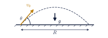
Fig. 81 Launch geometry of a pointlike projectile launched from the origin with initial speed \(v_0\) at angle \(\theta\) above the horizontal under uniform gravitational acceleration \(g\); the dashed curve is the resulting trajectory and \(R\) denotes the ground range.

---

Setup

Data only: gravity, the two per-unit-mass drag coefficients that select the Stokes and Newton regimes, and the default launch speed every flight here uses. The machinery this notebook is about is deliberately absent — you write the equations of motion rhs in Exercise 1, and in Exercise 2 the flight integrator fly together with its ground-impact event hit_ground, the range reader ground_range, and the dense resampler trajectory.

The Setup below holds this notebook’s data and instruments — nothing you are asked to build. It is collapsed so the building stays yours; expand it whenever you want the details.

Show code cell source

Hide code cell source

import numpy as np
from scipy.integrate import solve_ivp
import matplotlib.pyplot as plt
from matplotlib.animation import FuncAnimation

from ecp import validate
from ecp.animate import show

rng = np.random.default_rng(0)

# data: physical parameters (SI). Per-unit-mass drag coefficients, so mass
# drops out of the dynamics.
G = 9.81  # data: gravitational acceleration [m/s^2]
K_LIN = 0.5  # data: linear (Stokes) coefficient k = b/m   [1/s]
K_QUAD = 0.02  # data: quadratic (Newton) coefficient κ = c/m  [1/m]
V0 = 30.0  # data: default launch speed [m/s]

Exercise 1 — Implement the equations of motion

The dynamics are the two coupled second-order equations Eq. 99: each acceleration is gravity (vertical only) minus a damping rate \(k + \kappa|\mathbf v|\) times the corresponding velocity component. Writing them as a first-order system in the state \(\mathbf s = (x, v_x, y, v_y)\) is what lets a standard ODE solver integrate them, and carrying both drag coefficients in one function lets us select the vacuum, linear, or quadratic regime just by which one is non-zero. Every flight in the rest of the notebook is this one right-hand side, integrated. Switching both coefficients off must leave free fall — an acceleration of exactly \((0, -g)\) whatever the velocity — which is the first thing worth checking.

1. Write the right-hand side rhs(t, s, k_lin=0.0, k_quad=0.0, g=G), returning \((\dot x, \ddot x, \dot y, \ddot y)\) for Eq. 99: unpack the state, form the speed \(|\mathbf v| = \sqrt{v_x^2+v_y^2}\) (numpy.hypot) and the effective damping rate \(k + \kappa|\mathbf v|\), and return the derivative vector, remembering that only the vertical component carries the \(-g\) gravity term. Write this one yourself — the implementation is the lesson.

2. Evaluate it at a random state with both coefficients zero and confirm the drag-free limit.

Validation 1 — the drag-free limit is free fall

With both coefficients zero, the acceleration must be exactly \((0, -g)\) regardless of velocity. Evaluate rhs at a random state and check.

✓  drag-free limit is free fall   [max|Δ| = 0 (rtol=1e-12, atol=1e-09)]

True

Exercise 2 — Integrate to impact and plot a trajectory

With Eq. 99 in hand as a first-order system, an adaptive solver can carry the state forward in time. Two numerical ideas make the result clean: a terminal event stops the integration exactly at ground impact (\(y\) crossing zero on the way down) rather than at some arbitrary final time, and dense output lets us resample the few stored steps onto a fine grid so the plotted path is a smooth curve, not a polygon. The four pieces built here — the event, the launcher, the range reader, and the resampler — are the notebook’s workhorses: every exercise from here on calls them.

1. Write hit_ground(t, s, *args), the terminal event that returns the height \(y\) so the solver stops at the downward zero crossing, and fly(v0, theta_deg, k_lin, k_quad), which launches from the origin at speed \(v_0\) and angle \(\theta\) and integrates the rhs of Exercise 1 with scipy.integrate.solve_ivp (DOP853, dense_output=True, the event attached).

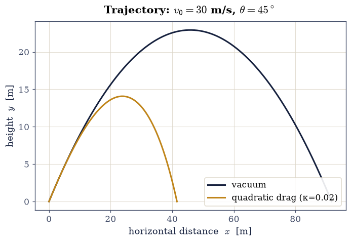
2. Write ground_range(sol), which reads the located impact distance off the event, and trajectory(sol, n), which resamples the dense output onto \(n\) evenly spaced times between launch and landing.

3. Overlay the vacuum and quadratic-drag paths for the same launch (\(v_0 = 30\) m/s, \(\theta = 45°\)): drag visibly shortens both the reach and the height.

4. Animate the two projectiles flying side by side (the worked solution below, FuncAnimation), then confirm with a check that the drag flight lands shorter.

A worked animation — the two flights, side by side

The static overlay shows the paths; an animation shows the motion. We sample both flights on a common clock (each on its own dense output up to its own landing time) and watch the drag projectile fall behind and land first. This is the worked example for the two-animation rule; you build the second one in Exercise 8.

Once Loop Reflect

Fig. 82 Animation of two projectiles launched together from the origin at speed \(v_0=30\) m/s and angle \(\theta=45^\circ\): one in vacuum (blue) and one under quadratic drag with coefficient \(\kappa=0.02\) m\(^{-1}\) (orange). Filled markers are the instantaneous positions and the trailing curves are the paths; the drag projectile lands first and shorter.

Validation 2 — drag shortens the range

Same launch, drag on: the quadratic flight must land closer than the vacuum flight. This checks the physics carried by the animation (the relative reach), not the drawing code.

✓  drag shortens the range at 45°   [R_quad=41.55 m < R_vac=91.74 m]

True

Exercise 3 — Vacuum range vs. the analytic parabola

The vacuum limit is the one place the trajectory has an elementary closed form: the range obeys Eq. 100. That makes it the natural correctness check on the whole pipeline: solver, event location, and ground_range together must reproduce a formula we know exactly.

1. With drag off, compute the range at \(\theta = 30°, 45°, 60°\) with the fly and ground_range you wrote in Exercise 2.

2. Compare each to \(R = v_0^2 \sin 2\theta / g\) from Eq. 100. (Verified to \(\sim10^{-15}\) with the tight solver + event location; \(10^{-4}\) is a safe ceiling.)

θ=  30°   R_num= 79.4519 m   R_analytic= 79.4519 m
θ=  45°   R_num= 91.7431 m   R_analytic= 91.7431 m
θ=  60°   R_num= 79.4519 m   R_analytic= 79.4519 m

✓  vacuum range matches v0^2 sin2θ/g   [max|Δ| = 1.42109e-13 (rtol=0.0001, atol=1e-09)]

True

Exercise 4 — Range vs. launch angle for all three regimes

Once range is a function we can evaluate at any angle, the whole curve \(R(\theta)\) is within reach, and Eq. 100 is only the vacuum member of the family. Plotting all three regimes together shows what drag does to the shape, not just to a single number.

1. Sweep the launch angle on a fine grid — your Exercise 2 fly and ground_range at every angle — and plot \(R(\theta)\) for vacuum, linear, and quadratic drag on one axes, marking each peak.

2. Note the shape: the vacuum curve is symmetric about its \(45°\) peak (the maximum of Eq. 100); the drag curves are lower and lean left — a first look at the optimal-angle shift made quantitative in Exercise 7.

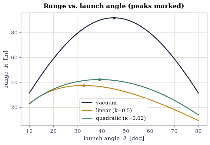
✓  vacuum optimum is 45°   [got 45 vs expected 45 (rtol=1e-06, atol=0.5)]

True

Exercise 5 — Linear drag matches its closed form

Turning off the quadratic term decouples the two components and leaves a linear system: the one case with drag that integrates by hand, giving the closed form Eq. 101. That exact solution is a second, independent check on the integrator: now with a drag term actually switched on.

1. Integrate the Stokes case (\(k = 0.5\), \(\kappa = 0\)) — the rhs you wrote in Exercise 1 — with scipy.integrate.solve_ivp (DOP853, dense_output=True).

2. Compare \(x(t)\) and \(y(t)\) to Eq. 101 at several times. (We integrate without the ground event so the comparison runs past the landing point, where the analytic solution still holds.)

 t [s]   x_num      x_ana      y_num      y_ana
  0.2    4.03741    4.03741    3.84759    3.84759
  0.5    9.38469    9.38469    8.25455    8.25455
  1.0   16.69349   16.69349   12.51323   12.51323
  1.5   22.38559   22.38559   13.65993   13.65993
  2.0   26.81860   26.81860   12.38301   12.38301

✓  linear drag matches closed form   [max|Δ| = 3.58472e-10 (rtol=1e-05, atol=1e-09)]

True

Exercise 6 — Quadratic terminal velocity

The quadratic case has no elementary closed form for the full trajectory, but one number survives exactly: in free fall the speed grows until drag balances gravity, fixing the terminal velocity Eq. 102. It is the checkable fingerprint of the nonlinear regime.

1. Drop an object from rest under quadratic drag (\(\kappa = 0.02\)) and integrate your Exercise 1 rhs long enough (~60 s, scipy.integrate.solve_ivp) for \(v_y\) to flatten.

2. Confirm the asymptote equals \(-\sqrt{g/\kappa}\) from Eq. 102. (Verified to \(\sim10^{-10}\); \(10^{-3}\) covers a shorter integration.)

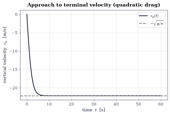
✓  quadratic terminal velocity = -√(g/κ)   [got -22.1472 vs expected -22.1472 (rtol=0.001, atol=1e-09)]

True

Exercise 7 — Why the optimal angle drops below 45°

The payoff. In vacuum the optimum is exactly \(45°\): the peak of Eq. 100. Drag breaks that symmetry: it penalises the long, slow, high-arc trajectories more than the flat ones, so the range-maximising angle slides below \(45°\).

1. For quadratic drag at \(v_0 = 30\) m/s, find the range-maximising angle on a fine grid (your Exercise 2 fly and ground_range again, then numpy.argmax over the swept ranges) and confirm it falls below the vacuum’s \(45°\) optimum.

2. Track the optimum across launch speeds and watch it drop further as \(v_0\) rises.

quadratic-drag optimum at v0=30 m/s:  θ ≈ 39°

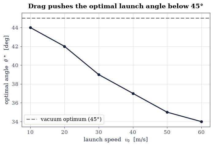
✓  drag lowers the optimal launch angle   [optimal θ ≈ 39° (vacuum is 45°)]

True

Exercise 8 — The approach to terminal velocity, across drag strengths

Exercise 6 measured the terminal velocity at one drag coefficient; here we map how the approach depends on \(\kappa\). Dropped from rest under quadratic drag, each \(v_y(t)\) flattens toward its own asymptote \(-\sqrt{g/\kappa}\) of Eq. 102: stronger drag means a lower terminal speed, reached sooner. This is a comparison plot, not an animation: the lesson is how the family of curves differ, which a still figure shows at a glance (a single curve creeping toward a line in real time would only obscure it).

1. For each \(\kappa \in \{0.02, 0.05, 0.10\}\,\mathrm{m^{-1}}\), drop from rest and integrate \(v_y(t)\) — your Exercise 1 rhs again — with scipy.integrate.solve_ivp on a fine grid long enough to flatten.

2. Plot the three \(v_y(t)\) together with their asymptotes \(-\sqrt{g/\kappa}\).

3. The validation checks each curve’s final velocity against Eq. 102.

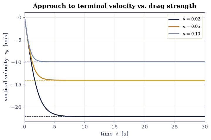
Fig. 83 Vertical velocity \(v_y(t)\) of an object dropped from rest under quadratic drag, for three drag coefficients \(\kappa\): each curve flattens to its own terminal velocity \(-\sqrt{g/\kappa}\) (matching dashed line) where gravity balances drag, with stronger drag giving a lower terminal speed reached sooner.

Validation 8 — every curve reaches its predicted terminal velocity

Each drop must flatten to the terminal velocity Eq. 102 for its own \(\kappa\). The check compares all three final velocities to \(-\sqrt{g/\kappa}\).

✓  each fall reaches its terminal velocity -√(g/κ)   [max|Δ| = 1.25922e-10 (rtol=0.001, atol=1e-09)]

True

Notebook summary

• Projectile motion integrated to impact (scipy.integrate.solve_ivp with a ground event) across three drag regimes: the vacuum range matched \(v_0^2\sin2\theta/g\) with a \(45°\) optimum, and the drag-free limit recovered free fall.

• Linear drag matched its closed form; the quadratic terminal velocity \(\sqrt{mg/c}\); the optimal launch angle dropping below \(45°\) as drag grows; and the approach to terminal speed.

Outlook

• Targeting (a shooting problem). With drag on, find the launch angle that makes the projectile pass through a given target \((x_\star, y_\star)\) by root-finding on the miss distance: there are generally two solutions, a flat and a lofted shot.

• Reynolds-number crossover. Estimate where linear vs. quadratic drag dominates for a real ball, and check the per-unit-mass coefficients used here against \(b, c\) from the size, speed, and air properties.

• Wind. Add a constant horizontal wind by evaluating the drag on the air-relative velocity \(\mathbf v - \mathbf v_\mathrm{wind}\), and watch the range become asymmetric in launch direction.

References

[Nol16]

Wolfgang Nolting. Theoretical Physics 1: Classical Mechanics. Springer, 2016. Grundkurs Theoretische Physik 1.

[Tay05]

John R. Taylor. Classical Mechanics. University Science Books, 2005.

Take this notebook with you

Use the download button (↓) in the toolbar above to save this notebook and run it yourself. The published notebooks ship without worked solutions; if you would like the reference solutions — to teach from or to check your own work — get in touch: hello@ramador.me.