4.2 The Lorentz Transformation, Derived

4.2 The Lorentz Transformation, Derived#

    Elementary Computational Physics
  

Volume IV — Special Relativity Notebook 4.2

From two postulates to the equations of spacetime: demanding that light keep the same speed in every frame forces a unique transformation of space and time, and time dilation, length contraction, and the relativistic addition of velocities all follow.

Level · intermediate • Est. · 110–140 min

    Raymond Amador
    v1.4.0  ·  2026-07-31  · 
          CC BY 4.0 (text) / MIT (code)
  

Notebook overview#

§4.1 ended with a transformation handed to us, the Lorentz transformation, asserted to be the map that keeps the speed of light the same for every observer. Here we earn it. Starting from nothing but the two postulates of §4.1 and the requirement that space and time be homogeneous, we write down the most general linear map between inertial frames and let the postulates fix its four coefficients. They leave no freedom: the transformation is forced, not chosen, and out of it fall time dilation, length contraction, and the relativistic rule for adding velocities, each as a theorem rather than a preview.

The strategy is to make every claim computational. We build the linear ansatz, impose the three physical conditions, and read off that the coefficients must be \(A=E=\gamma\), \(B=-\gamma v\), \(D=-\gamma v/c^2\). We then transform a light ray and watch it stay at \(c\); transform a stationary clock and watch its time stretch by \(\gamma\); transform a rod measured simultaneously and watch it shrink by \(1/\gamma\); and transform a velocity to recover the addition law that caps every sum at \(c\). Two structural gifts close the notebook: Lorentz boosts compose as a group, and in the rapidity parameter \(\varphi=\operatorname{arctanh}(v/c)\) a boost becomes a simple hyperbolic rotation whose parameters add. That last observation is the seed of the Minkowski geometry of §4.3.

A note on the relationship to Volume III. The capstone §3.12 used this transformation to rewrite electrodynamics in covariant form, taking it as given. Here it runs the other way: we derive the same map from physical principles, so that what §3.12 borrowed is now derived in full.

Everything is in SI units, with \(c=1/\sqrt{\mu_0\varepsilon_0}=2.998\times10^8\,\)m/s. Most figures are clean stills, but one effect, the contraction of a moving rod as its speed sweeps from rest toward \(c\), is genuine parametric motion, so it is animated; the spacetime-diagram view of the transformation is saved for §4.3.

How to read the checks. Each exercise closes with a validate call against an independent fact: the derived coefficients equal \(\gamma\) and \(-\gamma v\); the light ray stays at \(c\); the interval \(-(ct)^2+x^2\) is unchanged; the dilation is exactly \(\gamma\), the contraction exactly \(1/\gamma\); \(c\oplus0.5c=c\); two boosts compose into one; rapidities add. A ✓ is strong evidence; a ✗ is a prompt to locate the discrepancy, not a verdict.

Scope. A derivation of the transformation and its immediate kinematic consequences; the geometric picture (Minkowski diagrams, four-vectors) is §4.3 and the paradoxes are §4.4. See Einstein 1905 []; Nolting, Theoretical Physics 4 [Nol17]; Taylor & Wheeler, Spacetime Physics [TW92]; and §4.1 (the postulates) and §3.12 (which used this transformation).

Theory in brief#

What we require#

We seek a coordinate transformation \((t,x)\to(t',x')\) between two inertial frames in relative motion \(v\) that meets four demands,

(333)#\[\text{(i) linear} \quad \text{(ii) } S' \text{ origin moves at } v \text{ in } S \quad \text{(iii) } c \text{ invariant} \quad \text{(iv) } \to \text{Galileo as } v\ll c .\]

Linearity (i) follows from the homogeneity of space and time, no point or instant is special, so straight worldlines map to straight worldlines. Condition (ii) ties the map to the relative velocity, and (iii) is the second postulate of §4.1. Condition (iv) is the correspondence principle: whatever we find must contain Newton.

The derivation#

Write the most general linear map,

(334)#\[x'=A\,x+B\,t, \qquad t'=D\,x+E\,t .\]

Imposing (ii) — the point \(x'=0\) moves as \(x=vt\) — gives \(B=-Av\). Imposing (iii) — a light ray \(x=ct\) must map to \(x'=ct'\), and a left-going ray \(x=-ct\) to \(x'=-ct'\) — fixes \(E=A\) and \(D=-Av/c^2\). A final symmetry requirement, that the inverse transformation (replace \(v\to-v\)) undo the forward one, pins the remaining constant to \(A=\gamma\). The coefficients are forced:

(335)#\[A=E=\gamma, \quad B=-\gamma v, \quad D=-\frac{\gamma v}{c^2}, \qquad \gamma=\frac{1}{\sqrt{1-v^2/c^2}},\]

giving the Lorentz transformation \(t'=\gamma(t-vx/c^2)\), \(x'=\gamma(x-vt)\). For \(v\ll c\), \(\gamma\to1\) and it collapses to the Galilean \(t'\approx t\), \(x'\approx x-vt\).

The invariant interval#

The transformation preserves the spacetime interval,

(336)#\[s^2=-(ct)^2+x^2=-(ct')^2+x'^2 ,\]

the quantity all observers agree on even as \(t\) and \(x\) separately change. This is the geometric heart of relativity, developed as a pseudo-distance in §4.3.

Time dilation#

A clock at rest in \(S'\) (\(dx'=0\)) ticks off proper time \(d\tau\); the coordinate time in \(S\) is

(337)#\[dt=\gamma\,d\tau > d\tau .\]

Moving clocks run slow, by exactly \(\gamma\). The cosmic-ray muon reaches the ground only because its clock is dilated.

Length contraction#

A rod at rest in \(S'\) has proper length \(L_0\); measuring both ends simultaneously in \(S\) (\(dt=0\)) gives

(338)#\[L=\frac{L_0}{\gamma} < L_0 .\]

Moving rods are shorter, by exactly \(1/\gamma\). The two end-measurements simultaneous in \(S\) are not simultaneous in \(S'\) — the relativity of simultaneity of §4.1 is what dissolves the apparent paradox.

Relativistic velocity addition#

Differentiating the transformation, a velocity \(u\) in \(S\) becomes

(339)#\[w=\frac{u+v}{1+uv/c^2}\]

in the frame boosted by \(v\). Velocities no longer simply add; the result never exceeds \(c\), and \(c\oplus(\text{anything})=c\). The Galilean \(u+v\) is the low-speed limit.

Two structural gifts#

Finally, the transformation has a deeper shape,

(340)#\[\Lambda(v_2)\,\Lambda(v_1)=\Lambda(v_1\oplus v_2), \qquad \varphi=\operatorname{arctanh}(v/c), \quad \varphi_{\rm tot}=\varphi_1+\varphi_2 .\]

Boosts compose (closure: two boosts make one — the Lorentz group), and in the rapidity \(\varphi\) a boost is a hyperbolic rotation whose parameters add linearly where velocities do not. This is a direct preview of the Minkowski geometry of §4.3.

Setup#

Data and instruments only: the CODATA constants that fix \(c=1/\sqrt{\mu_0\varepsilon_0}\), the series palette, and the Lorentz factor \(\gamma(v)=1/\sqrt{1-v^2/c^2}\) — the one-line definition introduced in §4.1 and the independent yardstick every result below is checked against. This notebook’s own machinery is not here: you write the transformation itself, lorentz, in Exercise 2, the velocity-addition law vel_add in Exercise 6, and the boost matrix boost_matrix in Exercise 7. Deriving those three is the entire notebook, so none of them is handed over. No randomness appears anywhere in this notebook.

The Setup below holds this notebook’s data and instruments — nothing you are asked to build. It is collapsed so the building stays yours; expand it whenever you want the details.

Exercise 1 — Deriving the transformation (worked)#

This is the centerpiece: we do not assert the Lorentz transformation, we force it. Start from the most general linear map Eq. 334, \(x'=Ax+Bt\), \(t'=Dx+Et\), and impose the three physical conditions of Eq. 333. The origin of \(S'\) moving at \(v\) gives \(B=-Av\); demanding a light ray \(x=\pm ct\) map to \(x'=\pm ct'\) gives \(E=A\) and \(D=-Av/c^2\); and the inverse-symmetry requirement pins \(A=\gamma\). The coefficients are then completely determined Eq. 335. We did not choose these equations; the postulates left no other option, and the two checks below are what “no other option” means numerically.

Build the derived coefficient matrix as an explicit numpy array \(\begin{psmallmatrix}\gamma & -\gamma v\\ -\gamma v/c^2 & \gamma\end{psmallmatrix}\) acting on \((x,t)\), apply it to a light ray \(x=ct\) with the matrix product @, and confirm the transformed ray still satisfies \(x'=ct'\).
Confirm the final step of the derivation — that inverse symmetry pins \(A=\gamma\) — by checking \(M(-v)\,M(v)=\mathbb 1\): the backward boost exactly undoes the forward one only for this normalisation.

derived coefficient matrix on (x, t):
  A = E = γ      = 1.250000
  B = −γv        = -2.2484e+08
  D = −γv/c²     = -2.5017e-09

transformed light ray: x'/t' = 2.997925e+08 m/s  (c = 2.997925e+08)
M(−v) M(v) − 1: max normalized residual = 2.65e-17  (A=γ is what makes this exact)

Validation 1#

✓  the derived transformation keeps light at speed c   [max|Δ| = 1.19209e-07 (rtol=1e-06, atol=1e-09)]
✓  the backward boost undoes the forward one, M(−v)M(v)=1 — the symmetry that forces A=γ   [got 2.65093e-17 vs expected 0 (rtol=1e-06, atol=1e-12)]

True

Exercise 2 — The Galilean limit (worked)#

A new theory must contain the old one where the old one worked. For everyday speeds the Lorentz factor is indistinguishable from \(1\), and the transformation reduces to the Galilean \(t'\approx t\), \(x'\approx x-vt\) Eq. 333. The deviation is governed by \(\gamma-1\approx\tfrac12(v/c)^2\), utterly negligible at human speeds, which is exactly why relativity stayed hidden for centuries. Taking that limit means having the transformation in hand as something callable, so this is where the coefficients forced in Exercise 1 become a function — the one every exercise from here on runs through.

Write lorentz(t, x, v), returning the coordinates \(t'=\gamma(t-vx/c^2)\), \(x'=\gamma(x-vt)\) Eq. 335 of an event \((t,x)\) in the frame boosted by \(v\), with \(\gamma\) from the Setup. Written with numpy arithmetic it accepts whole arrays of events as readily as single ones, which the later exercises rely on. Write this one yourself — the implementation is the lesson; this map is what the notebook is about.
For a fast train at \(v=30\,\)m/s, evaluate \(\gamma(v)\), compare the Lorentz-transformed event coordinates against the Galilean ones (your lorentz vs. plain numpy arithmetic \(x-vt\)), and confirm \(\gamma-1\) matches the estimate \(\tfrac12(v/c)^2\) to leading order. Relativity does not overturn Newton; it contains him.

v = 30.0 m/s:  γ = 1.000000000000005
  γ − 1            = 5.107e-15
  ½(v/c)² estimate = 5.007e-15
  Lorentz x' = 70.000000000 m   vs   Galilean x' = 70.000000000 m
  Lorentz t' = 1.000000000000 s   vs   Galilean t' = 1.000000000000 s

Validation 2#

✓  at everyday speeds γ≈1 and Lorentz→Galilean   [got 1 vs expected 1 (rtol=1e-06, atol=1e-12)]
✓  the deviation γ−1 matches ½(v/c)² to leading order (float64: ~2%)   [got 5.10703e-15 vs expected 5.00693e-15 (rtol=0.05, atol=0)]

True

Exercise 3 — The invariant interval (worked)#

Individual coordinates are frame-dependent, but one combination is not: the spacetime interval \(s^2=-(ct)^2+x^2\) Eq. 336 is the same in every frame. It is the relativistic replacement for “distance”, and its invariance is the geometric content of the whole theory, the quantity all observers agree on while disagreeing about \(t\) and \(x\) separately.

For the four stated events, transform each with the lorentz you wrote in Exercise 2 to a frame at \(v=0.8c\), and form \(s^2\) before and after as the explicit combination \(-(ct)^2+x^2\) in numpy.
Confirm the two agree event by event with np.allclose, even though the individual \(t\) and \(x\) change substantially.

event        s² before        s² after
           -2.695021e-01   -2.695021e-01
           -1.436888e+00   -1.436888e+00
           -6.737552e+00   -6.737552e+00
           -4.488797e-01   -4.488797e-01

intervals match: True

Validation 3#

✓  the spacetime interval is invariant under the Lorentz transformation   [max|Δ| = 3.33067e-16 (rtol=1e-09, atol=1e-09)]

True

Exercise 4 — Time dilation, derived (worked)#

Now we turn the preview of §4.1 into a theorem. A clock sitting at rest in \(S'\) advances only in time, \(dx'=0\), marking its proper time \(d\tau\). Inverting the transformation, the coordinate time elapsed in \(S\) is \(dt=\gamma\,d\tau\) Eq. 337: more than \(d\tau\), since \(\gamma>1\). The moving clock runs slow by exactly \(\gamma\). This is not an illusion of signalling; it is the geometry. Cosmic-ray muons, with a rest lifetime of \(2.2\,\mu\)s, reach the ground only because their clocks are dilated.

For a proper-time tick \(d\tau=1\,\)s, compute the coordinate time \(dt\) from the transformation itself — transform the two ends of the tick at fixed \(x'\) with the lorentz you wrote in Exercise 2 and difference them — at \(v=0.6c\), \(0.9c\), \(0.99c\), and confirm it equals \(\gamma\,d\tau\).
Plot the dilation factor \(\gamma(v)\) across all speeds, with the three worked speeds marked on the curve.

   v/c        dt = γ dτ (s)      γ
60        1.250000        1.2500
90        2.294157        2.2942
99        7.088812        7.0888

Validation 4#

✓  moving clocks run slow by exactly γ   [max|Δ| = 0 (rtol=1e-09, atol=1e-09)]
✓  γ(0.6c)=1.25   [got 1.25 vs expected 1.25 (rtol=1e-06, atol=1e-09)]

True

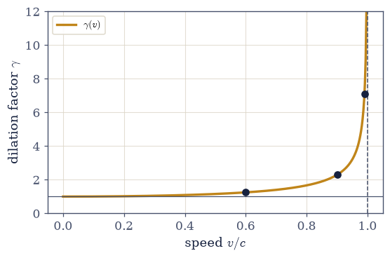
../../_images/b935ade01391e154c492eee2545b4349dd23cae3415f42d1821493c4a866739a.png — Fig. 351 Time dilation. A clock moving at speed \(v\) takes \(\gamma\) seconds of our coordinate time to advance one second of its own proper time, so the dilation factor \(\gamma(v)\) (amber) sits just above \(1\) for everyday speeds and diverges as \(v\to c\) (dashed). The three marked points are \(v=0.6c,0.9c,0.99c\), where \(\gamma=1.25,2.29,7.09\).#

Exercise 5 — Length contraction, derived (worked)#

Space contracts as time dilates. A rod of proper length \(L_0\) at rest in \(S'\) is measured in \(S\) by marking both ends at the same instant in \(S\) (\(dt=0\)); the transformation then gives \(L=L_0/\gamma\) Eq. 338. The subtlety is the simultaneity: the two end-markings simultaneous in \(S\) are not simultaneous in \(S'\), and this is precisely what reconciles the rod’s two observers (the lesson of §4.1). The contraction is real, reciprocal to the dilation, and animated below as the rod’s speed sweeps from rest toward \(0.9c\).

For a rest length \(L_0=1\,\)m at \(v=0.6c\), \(0.9c\), \(0.99c\), measure the contraction through the transformation just derived: both rod-end events must be simultaneous in \(S\), so pick the far end’s rod-frame event at \(t'=-vL_0/c^2\) and inverse-boost it with the lorentz you wrote in Exercise 2 (\(v\to-v\)); the mapped \(x\)-coordinate is the measured length. Confirm it equals \(L_0/\gamma\).
Animate the rod, deforming it continuously as \(v\) sweeps from rest to \(0.9c\).

   v/c      measured length (m)    L₀/γ (m)
60        0.8000            0.8000
90        0.4359            0.4359
99        0.1411            0.1411

Validation 5#

✓  the length measured through the derived transformation contracts by exactly 1/γ   [max|Δ| = 7.77156e-16 (rtol=1e-09, atol=1e-09)]

True

Fig. 352 Length contraction, animated. A rod of proper length \(L_0=1\,\)m (faint outline) is shown as its speed sweeps from rest to \(0.9c\); the solid amber bar is the length \(L=L_0/\gamma\) an observer in \(S\) measures, shrinking to \(0.44\,\)m at \(0.9c\). The contraction is reciprocal to the time dilation of the previous exercise: where clocks slow by \(\gamma\), lengths shrink by \(1/\gamma\).#

Exercise 6 — Relativistic velocity addition (worked)#

If a bullet is fired at \(u\) inside a ship moving at \(v\), the Galilean answer \(u+v\) can exceed \(c\), which the postulates forbid. Differentiating the transformation gives the correct rule \(w=(u+v)/(1+uv/c^2)\) Eq. 339, which bends every sum back below \(c\) and returns exactly \(c\) whenever either input is \(c\). The denominator is the whole story: negligible at low speed, decisive near \(c\).

Write vel_add(u, v), returning the combined speed \(w=(u+v)/(1+uv/c^2)\) Eq. 339; like lorentz it should work elementwise on numpy arrays, which Exercise 9 will use.
Tabulate \(0.5c\oplus0.5c\), \(0.9c\oplus0.9c\), and \(c\oplus0.5c\), and confirm the first is \(0.8c\), the second \(0.994c\), and the third exactly \(c\).
Plot \(w(u)\) for a fixed \(v=0.6c\) against the Galilean straight line \(u+v\), to see the asymptote at \(c\).

0.5c ⊕ 0.5c = 0.8000 c
0.9c ⊕ 0.9c = 0.9945 c
  c  ⊕ 0.5c = 1.0000 c  (exactly c)

Validation 6#

✓  adding any velocity to c still gives c   [got 2.99792e+08 vs expected 2.99792e+08 (rtol=1e-09, atol=1e-09)]
✓  0.5c ⊕ 0.5c = 0.8c, below c   [got 2.39834e+08 vs expected 2.39834e+08 (rtol=1e-09, atol=1e-09)]

True

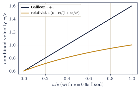
../../_images/0cdda59fed8c9204bf18d461c6d8ceeed2808aa9e6806a275a37d8ce15b7243f.png — Fig. 353 Relativistic velocity addition. Combining a velocity \(u\) with a fixed \(v=0.6c\) by the relativistic rule (amber) bends every sum back below the speed limit \(c\) (dashed), approaching but never reaching it. The Galilean sum \(u+v\) (dark) shoots past \(c\) without hesitation. The two agree only at low speed, where the denominator \(1+uv/c^2\approx1\).#

Exercise 7 — Boosts form a group (student)#

The transformations have an algebraic shape: apply one boost, then another, and the result is again a single boost Eq. 340. This closure is what makes the Lorentz boosts a group (the Lorentz group, explored in §4.3), and the speed of the combined boost is exactly the velocity-added speed of Exercise 6, the two structures locking together. Composition is cleanest in matrix form, where “apply one boost, then another” is a matrix product, so the transformation is needed once more as a matrix on the column \((ct,x)\) — the same coefficients as Exercise 1, in the symmetric coordinates where both entries carry \(\beta=v/c\).

Write boost_matrix(v), returning the \(2\times2\) array \(\begin{psmallmatrix}\gamma & -\gamma\beta\\ -\gamma\beta & \gamma\end{psmallmatrix}\) that acts on \((ct,x)\) Eq. 340, with \(\beta=v/c\) and \(\gamma\) from the Setup. Write this one yourself — the implementation is the lesson: every composition below is a product of these matrices.
Compose two boosts \(v_1=0.5c\) and \(v_2=0.7c\) by the matrix product boost_matrix(v2) @ boost_matrix(v1), and confirm with np.allclose that it equals a single boost at the velocity-added speed boost_matrix(vel_add(v1, v2)), using the vel_add you wrote in Exercise 6.

v1 = 0.5c, v2 = 0.7c   →   v1 ⊕ v2 = 0.8889 c
boost(v2) @ boost(v1):
[[ 2.18282063 -1.940285  ]
 [-1.940285    2.18282063]]
boost(v1 ⊕ v2):
[[ 2.18282063 -1.940285  ]
 [-1.940285    2.18282063]]

they are equal: True

Validation 7#

✓  two boosts compose into one — the Lorentz boosts form a group

True

With your assistant

Ask your assistant for a function returning the boost matrix \(\Lambda(v)\) in any dimension it likes — then apply the one gate every claimed Lorentz transformation must pass, whoever wrote it: \(\Lambda^{\mathsf T}\eta\,\Lambda = \eta\) to machine precision, the interval invariance of Exercise 3 in matrix form. One line of numpy.allclose settles what no amount of reading the code can. The check is yours.

Exercise 8 — Rapidity: the parameter that adds (student)#

Velocities add awkwardly, but there is a parameter that adds the way Galileo expected: the rapidity \(\varphi=\operatorname{arctanh}(v/c)\) Eq. 340. Composing two boosts simply adds their rapidities, \(\varphi_1+\varphi_2\), and inverting, \(v=c\tanh\varphi\), recovers the velocity-addition result. In rapidity the boost matrix becomes \(\begin{psmallmatrix}\cosh\varphi & -\sinh\varphi\\ -\sinh\varphi & \cosh\varphi\end{psmallmatrix}\), a hyperbolic rotation, the very form that makes a boost look like a rotation of spacetime in §4.3.

Compute the rapidities of \(v_1=0.5c\) and \(v_2=0.7c\) with np.arctanh, add them, and confirm with \(c\tanh(\varphi_1+\varphi_2)\) via np.tanh that the result equals the velocity-added speed from the vel_add you wrote in Exercise 6.
Plot \(v=c\tanh\varphi\) and watch it saturate at \(c\) as \(\varphi\to\infty\).

φ1 = arctanh(0.5) = 0.549306
φ2 = arctanh(0.7) = 0.867301
φ1 + φ2           = 1.416607
c·tanh(φ1+φ2) = 0.888889 c
vel_add(v1,v2) = 0.888889 c

Validation 8#

✓  rapidities add linearly where velocities do not   [got 2.66482e+08 vs expected 2.66482e+08 (rtol=1e-09, atol=1e-09)]

True

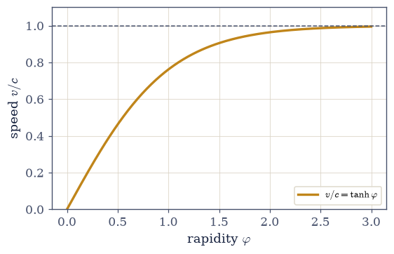
../../_images/a3c38b44d615d898c7381b423f4d77a6eb8738930e32e1421afb9a9d2385e6b7.png — Fig. 354 Rapidity, the additive parameter. A boost’s velocity is \(v=c\tanh\varphi\) (amber), so as the rapidity \(\varphi\) grows without bound the speed saturates at \(c\) (dashed) and never crosses it. Because composing boosts simply adds rapidities, the speed limit is built into the geometry: no finite sum of rapidities can push \(\tanh\) past \(1\). In \(\varphi\) a boost is a hyperbolic rotation, the seed of the Minkowski picture of §4.3.#

Exercise 9 — Everything from two postulates#

Stand back and see what has been built. From the two postulates of §4.1 and nothing else, the linear ansatz collapsed to a unique transformation; from that transformation fell time dilation, length contraction, and the velocity-addition law; and the transformation revealed a group structure whose natural parameter, the rapidity, adds linearly. No step required a new assumption. Two sentences of postulate, and the whole of relativistic kinematics follows.

What §3.12 borrowed as a tool, this notebook has derived.

Confirm the synthesis in one combined check: across a sweep of pair velocities, the speed from the vel_add you wrote in Exercise 6 never exceeds \(c\) (a numpy array comparison), the single guarantee that ties the velocity law, the group closure, and the rapidity saturation together.

largest |w| over all pairs: 0.999949 c
every relativistic sum stays below c: True
derived, not assumed: the transformation, dilation, contraction, addition,
the group, the rapidity — all from the two postulates of §4.1

Validation 9#

✓  no relativistic sum of velocities ever exceeds c — the speed limit is structural

True

Notebook summary#

The derivation Eq. 334, Eq. 335: the general linear map plus the three conditions (linearity, \(S'\) origin at \(v\), \(c\) invariant) force the coefficients to \(A=E=\gamma\), \(B=-\gamma v\), \(D=-\gamma v/c^2\); the transformation is not chosen but compelled, and the transformed light ray stays at \(c\) to machine precision.
Galilean limit Eq. 333: at \(v=30\,\)m/s, \(\gamma-1\approx5\times10^{-15}\) matches \(\tfrac12(v/c)^2\); relativity contains Newton.
Invariant interval Eq. 336: \(-(ct)^2+x^2\) is unchanged event by event under the transformation, the geometric quantity all observers share.
Dilation and contraction Eq. 337, Eq. 338: derived, not asserted — \(dt=\gamma\,d\tau\) (\(\gamma=1.25,2.29,7.09\) at \(0.6c,0.9c,0.99c\)) and \(L=L_0/\gamma\) (a \(1\,\)m rod measured at \(0.44\,\)m at \(0.9c\)), reciprocal faces of one factor.
Velocity addition Eq. 339: \(w=(u+v)/(1+uv/c^2)\) gives \(0.5c\oplus0.5c=0.8c\), \(0.9c\oplus0.9c=0.994c\), \(c\oplus0.5c=c\) exactly, capped at \(c\).
Group and rapidity Eq. 340: \(\Lambda(v_2)\Lambda(v_1)=\Lambda(v_1 \oplus v_2)\) (closure, by np.allclose), and \(\varphi=\operatorname{arctanh}(v/c)\) adds linearly with \(v=c\tanh\varphi\) saturating at \(c\) — the hyperbolic-rotation view that opens §4.3.

Outlook#

The geometric picture (§4.3). Minkowski spacetime, the interval as a pseudo-distance, boosts as the hyperbolic rotations glimpsed here in rapidity, and four-vectors, where the relativity computational toolkit (the metric, np.einsum index work) is built.
The paradoxes, resolved by computation (§4.4). The twin paradox and the pole-and-barn, dissolved by tracking worldlines through the transformation just derived.
Relativistic dynamics and \(E=mc^2\) (§4.5–§4.7). Four-momentum and the energy–mass relation, returning to the field tensor \(F^{\mu\nu}\) of §3.12.
The Lorentz group. The closure shown here is one face of a richer structure, rotations and boosts together, with their generators (a pointer, developed in §4.3).
Cross-reference §3.12. The transformation used there to build the covariant Maxwell equations is the one this notebook has now derived from physical principles.

Take this notebook with you

Use the download button (↓) in the toolbar above to save this notebook and run it yourself. The published notebooks ship without worked solutions; if you would like the reference solutions — to teach from or to check your own work — get in touch: hello@ramador.me.