


5.10 The Ising Model: Emergence, Symmetry Breaking, and Universality#
Notebook overview#
This is the conceptual climax of the volume. Everything we built — counting microstates (§5.1), the Boltzmann weight (§5.4), the Metropolis algorithm (§5.8), the fluctuation–response relations (§5.9) — converges here on a single, almost embarrassingly simple model, and out of it comes something none of the parts contained: a sharp phase transition, and the spontaneous birth of order from a law that has no preferred direction. The Ising model is a grid of spins that each point up or down and prefer to agree with their neighbours. That is the entire rule. Yet below a critical temperature the grid suddenly chooses — it magnetizes, picking one of two perfectly equivalent directions — and this collective decision, made by no single spin, is emergence in its cleanest form.
We are after the meaning of this, not the numbers. There is a magnificent quantitative theory of the Ising model — Onsager’s exact solution, the transfer matrix, finite-size scaling, the critical exponents, cluster algorithms — and it is developed in full in the Materials Modelling (MMM) course, where Ising is the vehicle for learning Monte Carlo because it can be solved exactly and checked against. We do not reproduce that here; we cross-reference it, and instead spend our effort on three ideas that the quantitative treatment rushes past:
Spontaneous symmetry breaking. The Hamiltonian is perfectly symmetric — flip every spin and the energy is unchanged — yet below \(T_c\) the equilibrium state is not symmetric. The law respects a symmetry the state violates.
Ergodicity breaking — the deep point, and the novel core of this notebook. A finite Ising magnet does not truly break the symmetry: given long enough, its magnetization flips sign. The familiar plots of \(|m|\) quietly hide this. True symmetry breaking — a permanently chosen direction — exists only in the limit \(N\to\infty\), and it happens by ergodicity breaking, the exact counterpart to the ergodicity we studied in §5.5.
Universality. The very same model is a magnet, a fluid at its critical point, a binary alloy — unrelated systems that share identical critical behaviour, because near a critical point the microscopic details wash out (Ising-type spins reach even further, to neural networks). It is why a toy explains reality.
The Metropolis algorithm of §5.8 is our microscope: we invoke it (we do not rebuild it) to watch the lattice order, to track the telltale sign-flipping, and to measure the susceptibility — which, as §5.9 promised, is a fluctuation that diverges at the critical point. By the end the whole arc of the volume will have closed: we began by counting microstates, and we end by watching order create itself.
How to read the checks. Each exercise closes with a
validatecall against an independent fact: the lattice orders below \(T_c\) and disorders above; the symmetric law yields a non-symmetric ordered state; a finite system’s magnetization flips sign, less and less often as it grows; the susceptibility (a §5.9 fluctuation) peaks at \(T_c\); the magnet-to-fluid mapping is exact; and a quench freezes in spontaneous order. A ✓ is strong evidence; a ✗ is a prompt to locate the discrepancy.Scope, and the bidirectional MMM link. This notebook is about concepts — emergence, symmetry breaking, ergodicity breaking, universality. All quantitative apparatus (the exact 1-D transfer matrix, Onsager’s 2-D solution, finite-size scaling, the critical exponents, the correlation length \(\xi(T)\), cluster algorithms, the Binder cumulant) lives in the Materials Modelling course and is referenced there, not derived here. The renormalization-group explanation of universality is the horizon beyond both. See Sethna, Statistical Mechanics; Goldenfeld, Lectures on Phase Transitions; and Notebooks §5.5 (ergodicity), §5.8 (Metropolis), §5.9 (the susceptibility fluctuation, the criticality bridge), §5.1/§5.4 (counting/Boltzmann).
Theory in brief#
The model and its symmetry#
Spins \(\sigma_i=\pm1\) sit on a lattice and prefer to align with their neighbours,
the simplest model of cooperation (MMM develops it fully). The one structural fact we need: \(E\) has a \(\mathbb{Z}_2\) symmetry — flip every spin, \(\sigma_i\to-\sigma_i\), and the energy is unchanged — so the two fully ordered states (all up, all down) are exactly degenerate. Whether the system respects that symmetry is the question of the notebook.
Spontaneous symmetry breaking#
Below a critical temperature \(T_c\) the system spontaneously magnetizes: it picks one of the two degenerate ordered states, and the symmetric \(m=0\) state becomes unstable,
This is spontaneous symmetry breaking: the law (the Hamiltonian) is symmetric, but the equilibrium state is not. Above \(T_c\) thermal agitation wins and \(m=0\). The order parameter \(m\) tells the phases apart. The Onsager benchmarks — \(T_c=2/\ln(1+\sqrt2)\approx2.269\,J/k\) and the exact magnetization with its \(\tfrac18\) exponent — are known results, derived in MMM/Onsager, not here.
Ergodicity breaking — the deep point#
Here is what a quick treatment hides. A finite Ising system below \(T_c\) does not truly break the symmetry: given enough time its magnetization flips sign, tunnelling between the two ordered states through a disordered fluctuation, so the long-time average of the signed \(m\) is zero — the symmetry is respected after all,
We plot \(|m|\) precisely to mask this finite-size flipping. True symmetry breaking — a permanently chosen sign — emerges only as \(N\to\infty\), where the free-energy barrier between the two states (proportional to the domain-wall area) makes the flip time diverge. The system then ceases to explore all of its accessible states — it is trapped in one symmetry sector. This is ergodicity breaking, the exact counterpart to the ergodicity of §5.5, and it is the mechanism behind every phase transition: how a symmetry that holds for every finite system can fail in the limit.
Criticality, fluctuations, and the §5.9 bridge#
Near \(T_c\) the magnetization fluctuations become enormous. The susceptibility is their measure — the fluctuation–response relation of §5.9 —
This is exactly the breakdown §5.9 foretold: at a critical point the fluctuations do not vanish as \(1/\sqrt N\), the response diverges, and the system becomes correlated over all length scales — the correlation length \(\xi\) diverges, and domains of every size appear at once (critical opalescence). We show this conceptually and visually; the quantitative \(\xi(T)\), the exponent \(\nu\), and finite-size scaling are MMM’s.
Universality#
Because the correlation length is huge at criticality, the system looks the same at every scale (scale invariance), and the microscopic details stop mattering — only the dimensionality and the symmetry survive,
So wildly different systems share identical critical behaviour: the Ising magnet, the lattice gas (the liquid–vapour critical point), and a binary alloy (order–disorder) fall into the same universality class — and the same Ising-type spins reach even further, into associative-memory neural-network models. A magnet losing its magnetization and a fluid at its critical point are, near criticality, the same model. Universality is why a stripped-down toy explains real, unrelated experiments — the deepest idea in the theory of phase transitions. (Its explanation, the renormalization group, is the horizon beyond both courses.)
Setup#
Data and instruments only. The data are the series palette with the two-colour map that renders a spin lattice, and Onsager’s exact \(T_c=2/\ln(1+\sqrt2)\) — a known result, quoted from the exact solution and not derived here. The instruments are the Metropolis machinery: one checkerboard sweep of the lattice and the driver that runs it and records the magnetization trace. The acceptance rule inside the sweep was built from scratch in §5.8, and this notebook is deliberate about invoking the sampler rather than rebuilding it — here it is the microscope, not the lesson, and the quantitative Ising craft (Onsager’s solution, finite-size scaling, cluster algorithms) belongs to the Materials Modelling course. What this notebook asks you to build is the measurement that exposes its central claim: the hysteresis flip counter of Exercise 3. Every simulation seeds its own generator where it is used.
The Setup below holds this notebook’s data and instruments — nothing you are asked to build. It is collapsed so the building stays yours; expand it whenever you want the details.
Exercise 1 — The model, its symmetry, and a first look at the transition (worked)#
We begin compactly, because the model and its mechanics belong to MMM; what we need is the picture. The rule is Eq. 435: spins on a grid, each \(\pm1\), with an energy that is lowered whenever neighbours agree. The single structural fact that will drive everything is the \(\mathbb{Z}_2\) symmetry — flipping all spins together costs no energy, so “all up” and “all down” are exactly equivalent. Now run the Metropolis algorithm of §5.8 at two temperatures and look (Fig. 454). Hot, the lattice is a structureless salt-and-pepper of up and down, with magnetization \(m\approx0\): thermal agitation overwhelms the alignment preference. Cold, the lattice has organized itself into large domains of a single sign, with \(|m|\) near one: the alignment preference has won. Somewhere between sits the critical temperature, \(T_c=2/\ln(1+\sqrt2)\approx 2.269\) (Onsager’s exact result, derived in MMM), where the change from disorder to order is sharp. A \(64\times64\) lattice run for 700 sweeps is large enough to show domains and short enough to be instant; half the sweeps are discarded as burn-in, since a run started from a random configuration needs time to forget it.
Part a) Run ising_metropolis on a \(64\times64\) lattice at \(T=1.6\) and again at \(T=3.5\), and
report the mean \(|m|\) over the post-burn-in sweeps for each.
Part b) Display the two final configurations side by side, and confirm \(|m|\) is large below \(T_c\) and near zero above.
Onsager T_c = 2/ln(1+√2) = 2.2692
T = 1.6 (below T_c): |m| = 0.980   → ordered (large domains)
T = 3.5 (above T_c): |m| = 0.030   → disordered (salt-and-pepper)
Validation 1#
✓ the system orders below T_c (|m| large) and disorders above it (|m| ≈ 0)
True
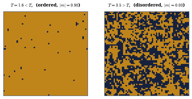
Fig. 454 The Ising transition, seen on the lattice. Left (\(T=1.6<T_c\)): the spins have organized into large domains of a single sign — the system is ordered, \(|m|\) near one, the alignment preference winning. Right (\(T=3.5>T_c\)): a structureless salt-and-pepper of up (amber) and down (ink), \(m\approx0\) — disordered, thermal agitation winning. The same local rule (neighbours prefer to align) produces both, depending only on temperature; the sharp change between them, at \(T_c\approx2.269\), is the phase transition this notebook is about.#
Exercise 2 — Spontaneous symmetry breaking (worked)#
Now we make the central concept precise. The Hamiltonian Eq. 435 is unchanged when we flip every spin — it has no preference between up and down — and yet below \(T_c\) the system ends up magnetized in one direction. How can a symmetric law produce an unsymmetric outcome? This is spontaneous symmetry breaking Eq. 436, and the word “spontaneous” is the point: nothing in the rules picks the direction, the system picks it itself, and which way it goes is decided by history (the initial condition, or the chance fluctuations as it cools). We can see the degeneracy directly: start the same cold system from “all up” and from “all down” and it settles into two mirror-image ordered states, \(+m_0\) and \(-m_0\), both equally valid solutions of the same symmetric problem (Fig. 455). Above \(T_c\) there is no such choice to make — the unique equilibrium state is the symmetric, disordered one with \(m=0\). The broken symmetry below \(T_c\) is not in the laws; it is in the state the laws permit the system to fall into. The measurement that shows this must be the signed mean magnetization, not \(|m|\): the absolute value would erase exactly the history-dependence at issue.
Part a) Run a \(48\times48\) lattice at \(T=1.6\) for 500 sweeps from an all-up start and again from an all-down start, discarding half as burn-in, and report the signed mean \(m\) of each.
Part b) Show the two final configurations side by side, and confirm they are oppositely magnetized — the same energy, the same physics, opposite choices.
the same symmetric Hamiltonian, two equivalent ordered states:
  started all-up   →  m = +0.979
  started all-down →  m = -0.980
the law has no preferred direction; the state chooses one — spontaneous symmetry breaking
Validation 2#
✓ the symmetric Hamiltonian yields a non-symmetric ordered state whose sign is set by history — spontaneous symmetry breaking
True
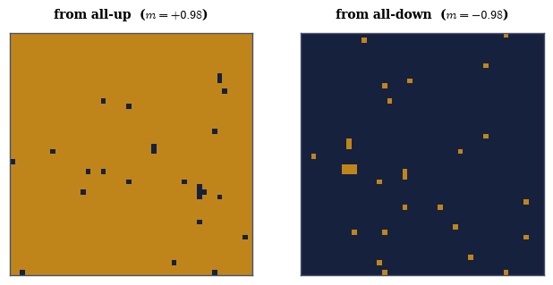
Fig. 455 Spontaneous symmetry breaking: two equal choices. The same cold system (\(T=1.6<T_c\)), started from all-up (left) and all-down (right), settles into oppositely-magnetized ordered states, \(+m_0\) and \(-m_0\). Both have identical energy and are equally valid equilibria of the same symmetric Hamiltonian — nothing in the rules prefers one, yet the system must pick. Which way it goes is set by history (here, the initial condition). The symmetry is unbroken in the law and broken in the state: that is what ‘spontaneous’ means.#
Exercise 3 — Ergodicity breaking: why a finite system never quite breaks the symmetry (worked)#
Here is the novel heart of the notebook, and the place where the honest story diverges from the tidy one. We just saw a finite cold lattice “choose” a magnetization sign — but watch it long enough and something disquieting happens: the sign flips. The whole magnet, fluctuation by fluctuation, tunnels through a disordered configuration and re-orders the other way, then back again (Fig. 456). Over a long run the signed magnetization spends equal time at \(+m_0\) and \(-m_0\), so its time average is zero Eq. 437 — the symmetry is respected after all. A finite Ising magnet does not truly break the symmetry. The plots of \(|m|\) that everyone shows, ours included, take the absolute value precisely to hide this flipping; they are a kindly lie. The signed magnetization tells the truth.
What rescues genuine symmetry breaking is size. To flip, the system must build a domain wall across itself, and the free-energy cost of that wall grows with the lattice (its area), so the time between flips grows explosively with \(N\) — and diverges as \(N\to\infty\). A macroscopic magnet would take longer than the age of the universe to flip, so it is, for all purposes, permanently stuck in the sector it chose. That trapping is ergodicity breaking: the system stops exploring all of its accessible states, the exact counterpart to the ergodicity of §5.5. It is how a symmetry that holds for every finite system fails in the limit — the mechanism of every phase transition.
Counting those flips honestly takes care. While the magnet reverses, \(m\) wanders about zero and crosses it many times, so a naive count of zero-crossings would report a burst of spurious flips for every real one. The cure is hysteresis, the Schmitt-trigger rule: declare the state \(+\) only once \(m\) has risen above \(+0.5\), declare it \(-\) only once \(m\) has fallen below \(-0.5\), and count a flip only when the declared state genuinely changes. Runs of 8000 sweeps at \(T=2.15\) (below \(T_c\)), the first 500 discarded, are long enough to catch many flips at \(L=6\) and almost none at \(L=16\); all three lattices are started fully ordered so that the run begins inside one sector and every flip counted is a real escape from it.
Part a) Write count_sign_flips(m, threshold=0.5), returning the number of sustained sign
reversals in a magnetization trace under the hysteresis rule above.
Write this one yourself — the implementation is the lesson: the threshold, not the sign of
\(m\), is what separates a genuine reversal from the noise of one in progress.
Part b) Track the signed \(m(t)\) for \(L=6\), \(10\) and \(16\) at \(T=2.15\), count the flips in each, and confirm the count collapses as the lattice grows.
Part c) Plot the three signed traces together, each labelled with its flip count.
L= 6 at T=2.15 (below T_c): sign flips = 34 (|m| = 0.863)
L=10 at T=2.15 (below T_c): sign flips = 10 (|m| = 0.844)
L=16 at T=2.15 (below T_c):  sign flips =   2   (|m| = 0.832)
the flip rate collapses with size — true symmetry breaking is a property of the N→∞ limit
Validation 3#
✓ a finite Ising magnet's magnetization flips sign over time, less and less often as it grows — symmetry is broken only as N→∞ (ergodicity breaking)
True
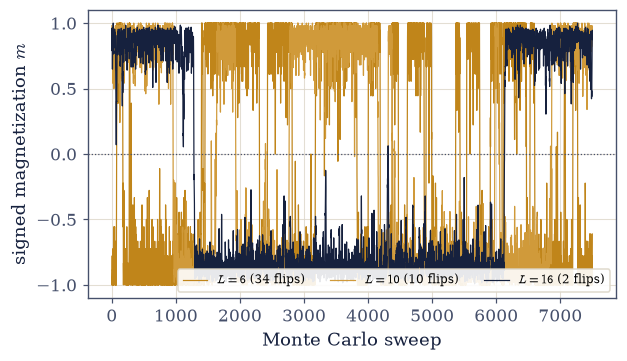
Fig. 456 Ergodicity breaking: the signed magnetization tells the truth. The signed \(m(t)\) for three lattice sizes at \(T=2.15<T_c\) over the same run. The small lattice (\(L=6\), amber) flips between the \(+\) and \(-\) ordered states freely — its long-time signed average is zero, so it respects the \(\mathbb{Z}_2\) symmetry. As the lattice grows the flips become rarer (\(L=10\), mid) and then almost cease (\(L=16\), dark), because the free-energy barrier to flip grows with size. A finite magnet never truly breaks the symmetry; the familiar \(|m|\) plot hides this by discarding the sign. True symmetry breaking — a permanently chosen direction — emerges only as \(N\to\infty\), when the flip time diverges and the system is trapped in one sector: ergodicity breaking, the counterpart to §5.5.#
Exercise 4 — Criticality and diverging fluctuations (worked)#
We now connect the transition to the fluctuation machinery of §5.9, and find that the bridge it built carries us exactly here. Near \(T_c\) the magnetization does not merely change its average — it fluctuates violently, as patches of order form and dissolve on every scale at once. The measure of those fluctuations is the susceptibility, and by the fluctuation–response relation of §5.9 it is \(\chi=N\operatorname{Var}(|m|)/kT\) Eq. 438 (we use \(|m|\) to factor out the finite-size sign-flipping of Exercise 3). Computed across temperature, \(\chi\) stays tiny deep in the ordered phase, then peaks sharply at \(T_c\) (Fig. 457) — and in the thermodynamic limit the peak becomes a true divergence. This is precisely the breakdown §5.9 foretold: a critical point is where the relative fluctuations do not vanish as \(1/\sqrt N\), where a response function diverges, and where the system becomes correlated across its entire size. The correlation length \(\xi\) diverges, and the lattice fills with domains of every size — the shimmer a real fluid shows at its critical point, called critical opalescence. The quantitative \(\xi(T)\) and the exponents that govern the divergence are MMM’s; the concept — fluctuations gone macroscopic — is the whole story. Fifteen temperatures spanning \(1.8\) to \(3.2\) on a \(32\times32\) lattice bracket \(T_c\approx2.269\) closely enough to place the peak; 1800 sweeps per temperature with 700 discarded leave enough post-burn-in samples for a variance to mean anything, since \(\chi\) is built from a fluctuation and a fluctuation needs statistics. Note the definition uses \(\operatorname{Var}(|m|)\), not \(\operatorname{Var}(m)\): the absolute value factors out the finite-size sign-flipping of Exercise 3, which would otherwise swamp the physical fluctuation.
Part a) Compute \(\chi=N\operatorname{Var}(|m|)/kT\) (with numpy.var) across the temperature
range, and take a snapshot at \(T_c\) on a larger, \(96\times96\) lattice.
Part b) Report the peak \(\chi\) and the temperature at which it falls, and confirm the peak sits near \(T_c\) and far above the deep-ordered value at \(T=1.8\).
Part c) Plot \(\chi(T)\) against temperature beside the critical snapshot, in which domains of every size should coexist.
susceptibility χ = N·Var(|m|)/kT  (L=32):
  peak χ = 21.2 at T = 2.30   (T_c = 2.27)
  deep-ordered χ(T=1.8) = 0.11   → χ jumps by ~190× toward T_c
the susceptibility is a §5.9 fluctuation–response function, and it diverges at criticality
Validation 4#
✓ the susceptibility — a fluctuation–response function (§5.9) — peaks at the critical point, where fluctuations stop vanishing as 1/√N
True
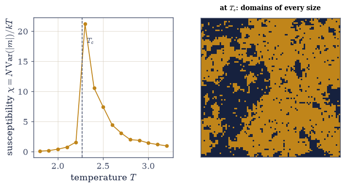
Fig. 457 Fluctuations diverge at the critical point. Left: the susceptibility \(\chi=N\operatorname{Var}(|m|)/kT\) — the magnetization fluctuation, the fluctuation–response function of §5.9 — against temperature. It is tiny deep in the ordered phase, then peaks sharply at \(T_c\approx2.269\) (dashed); in the thermodynamic limit the peak is a true divergence. Right: a snapshot at \(T_c\) — domains of every size coexist, the lattice correlated across its whole extent (the correlation length has diverged). This is the breakdown §5.9 foretold: a critical point is where fluctuations go macroscopic and response functions blow up. The exponents governing the divergence belong to MMM.#
Exercise 5 — Universality and the lattice-gas mapping (worked)#
We arrive at the idea that makes the Ising model matter far beyond magnetism. Why should a toy of \(\pm1\) spins tell us anything about real materials? Because of what happens to detail at a critical point. There the correlation length is enormous, so the system looks statistically the same whether you squint or zoom — it is scale invariant — and under that magnification the microscopic specifics (what the constituents are, the precise interaction) blur away. What survives is only the coarsest information: the dimensionality of space and the symmetry of the order parameter. Systems that agree on those fall into the same universality class and exhibit identical critical behaviour, with the same critical exponents, no matter how different they look up close.
The cleanest example is an exact change of variables Eq. 439: relabel a spin \(\sigma_i=\pm1\) as an occupation \(n_i=(1+\sigma_i)/2\in\{0,1\}\) — “up” becomes “an atom here”, “down” becomes “an empty site” — and the Ising magnet becomes a lattice gas. Its phase transition is then the liquid–vapour critical point of a fluid; the magnetization maps to the density difference between liquid and gas. The same algebra describes a binary alloy ordering, and the same Ising-type model even reaches associative-memory neural networks. So the curve along which a magnet loses its magnetization and the curve along which a fluid reaches its critical point are, near the critical point, governed by one model. This is why a stripped-down toy explains real, unrelated experiments — and why the Ising model is one of the most important models in physics. (The deep explanation, the renormalization group, is the horizon beyond this course.)
The claim to check is small and complete: because a spin takes only the two values \(\pm1\), the whole dictionary is two entries wide, and showing that \(n=(1+\sigma)/2\) and its inverse \(\sigma=2n-1\) return the original values on both of them is a proof, not a sample.
Part a) Map both spin values \(\sigma=\pm1\) to occupations \(n=(1+\sigma)/2\) and map them back with \(\sigma=2n-1\), printing the dictionary in both directions.
Part b) Confirm the occupations are exactly \(\{0,1\}\) and the round trip is the identity — the magnet and the lattice gas are literally the same model in two languages.
the Ising ↔ lattice-gas dictionary (an exact change of variables):
  spin σ        = [-1, 1]   (−1 = down,  +1 = up)
  occupation n  = [0, 1]   (0 = empty, 1 = atom)   via n = (1+σ)/2
  invert 2n−1   = [-1, 1]   (exact bijection: True)
→ a magnet and a fluid near their critical points are the same model — universality
Validation 5#
✓ the Ising-to-lattice-gas map σ ↔ n=(1+σ)/2 is an exact change of variables — a magnet and a fluid are the same model (universality)
True
Exercise 6 — The transition from the other side: a quench (student)#
To feel the order appear, we approach the transition the way nature usually does — by cooling. We take a hot, disordered configuration and suddenly drop the temperature below \(T_c\) (a quench), then watch (Fig. 458). At first the lattice is a fine speckle; almost immediately small aligned patches form, and then the domains coarsen — small ones are eaten by their neighbours, walls straighten and contract, and a single sign gradually takes over the lattice. Which sign wins is decided by the chance imbalance in the early fluctuations, and once a large domain has formed it is, by the ergodicity-breaking argument of Exercise 3, effectively frozen — the order is “locked in.” This is how a magnet cooled through its Curie point acquires a permanent magnetization, and how, more generally, spontaneous order crystallizes out of a symmetric disordered state as a system is taken across a phase transition. (How fast the domains coarsen, and the dynamics of the approach to equilibrium, is the non-equilibrium physics that §5.11 begins.)
A quench needs the sweep on its own rather than ising_metropolis, because the object of interest
is the sequence of configurations, not the magnetization trace: drive ising_sweep directly and
keep a copy of the lattice every third sweep. That means building the two checkerboard masks
yourself — the parity of \(i+j\) splits the lattice into the two colours. A \(64\times64\) lattice
started fully random and held at \(T=1.5\) has coarsened into a single dominant domain within about
120 sweeps.
Part a) Quench a random \(64\times64\) lattice to \(T=1.5\) for 120 sweeps, keeping a snapshot and the magnetization every third sweep.
Part b) Confirm the run began disordered (\(|m|\approx0\)) and ended magnetized — spontaneous order frozen in by cooling.
Part c) Animate the stored snapshots so the coarsening can be watched.
quench to T=1.5 (<T_c): |m| went from 0.019 (disordered) to 0.985 (ordered)
domains coarsened and a single sign took over — spontaneous order frozen in by cooling
Validation 6#
✓ a quench below T_c produces a magnetized state via domain coarsening — cooling through T_c freezes in spontaneous order
True
Fig. 458 Order crystallizing: a quench through \(T_c\) (animated). A hot, disordered lattice is suddenly cooled to \(T=1.5<T_c\). Out of the fine initial speckle, small aligned patches appear and then coarsen — small domains are swallowed, walls straighten, and one sign (amber or ink) gradually claims the whole lattice. Which sign wins is set by the chance imbalance of the early fluctuations; once a large domain forms it is effectively frozen (the ergodicity breaking of Exercise 3). This is how a magnet cooled through its Curie point acquires a permanent magnetization — spontaneous order, created by crossing a phase transition. The dynamics of the coarsening is the non-equilibrium story 5.11 opens.#
Exercise 7 — Emergence: the whole volume in one model (synthesis)#
Stand back and see what just happened, because it is the lesson the entire volume was built to deliver. The Ising model is where everything converged. The microstate counting of §5.1 and the Boltzmann weight of §5.4 defined it. The Metropolis algorithm of §5.8 sampled it. The fluctuation–response relations of §5.9 gave its susceptibility, and the ergodicity of §5.5 returned, inverted, as the ergodicity breaking that makes its symmetry breaking real. And out of those assembled parts came something that was in none of them: a sharp phase transition, spontaneous order from a symmetric law, and the universality that lets a toy of \(\pm1\) spins speak for real fluids and alloys. Emergence — qualitatively new collective behaviour arising from simple local rules — is the deepest lesson of statistical mechanics, and the Ising model shows it required all of the machinery, working together.
There is no new computation to run here; the convergence itself is the result. We began this volume by counting microstates, and we end it by watching order create itself. Nothing in a single spin knows what a phase transition is, yet together the spins break a symmetry their own law respects. That gap — between the local rule and the collective fact — is where physics becomes deep. For the quantitative craft (exact solutions, finite-size scaling, the critical exponents) the road leads to the Materials Modelling course; for how a system reaches these equilibrium states at all, and the arrow of time that points the way, 5.11 begins the non-equilibrium story.
With your assistant
Ask your assistant for a Metropolis variant of its own devising — a different proposal scheme, a different sweep order, a checkerboard update — and run it on this notebook’s lattice. The gate is statistical: it must reproduce the measured \(\langle|m|\rangle(T)\) and the susceptibility peak of this notebook within their error bars. Sampling algorithms differ; the physics may not. The check is yours.
Notebook summary#
The Ising model is the conceptual climax of the volume: collective order emerging from a symmetric local rule. We pursued its meaning (the quantitative apparatus is the Materials Modelling course’s).
The model and its symmetry Eq. 435: spins \(\pm1\) preferring to align, with a \(\mathbb{Z}_2\) symmetry making “all up” and “all down” degenerate.
Spontaneous symmetry breaking Eq. 436: below \(T_c\approx2.269\) the system magnetizes, choosing one of two equal directions — the law symmetric, the state not (verified: all-up and all-down starts give \(\pm m_0\)).
Ergodicity breaking Eq. 437: a finite magnet’s signed \(m\) flips sign (its time average is zero), and the flip rate collapses with size (\(L=6\) flips freely, \(L=16\) barely) — true symmetry breaking exists only as \(N\to\infty\), by trapping in one sector, the counterpart to the ergodicity of §5.5.
Criticality Eq. 438: the susceptibility \(\chi=N\operatorname{Var}(|m|)/kT\) (a §5.9 fluctuation–response function) peaks at \(T_c\) (verified \(\sim20\) vs \(\sim0.1\) deep ordered) and diverges in the limit — fluctuations gone macroscopic, the correlation length diverging.
Universality Eq. 439: scale invariance at criticality washes out microscopic detail, so the magnet, the lattice gas (the liquid–vapour critical point, via \(\sigma\leftrightarrow n=(1+\sigma)/2\)), the binary alloy, and more share one universality class.
Emergence — new collective behaviour from local rules — needed the whole volume, and the Ising model is where it all came together.
Outlook#
The quantitative Ising model — Materials Modelling (MMM). The exact 1-D transfer matrix, Onsager’s 2-D solution, finite-size scaling, the critical exponents, the correlation length \(\xi(T)\), cluster algorithms, the Binder cumulant — the craft of extracting numbers, developed in full in MMM. This is the bidirectional link: ECP for the concepts, MMM for the computation.
The renormalization group. The explanation of universality and scale invariance — why microscopic detail washes out at criticality — the horizon beyond both courses.
A taste of non-equilibrium (5.11). How a system reaches equilibrium at all, the dynamics of coarsening and relaxation, and the arrow of time behind the equilibrium states this volume described.
The quantum Ising model (Volume VII). The transverse-field Ising model and its quantum phase transition — order destroyed by quantum, not thermal, fluctuations — once Volume VI builds the quantum mechanics.
Cross-reference §5.5 (ergodicity), §5.8 (Metropolis), §5.9 (the susceptibility fluctuation, the criticality bridge), §5.1/§5.4 (counting and the Boltzmann weight).