


2.2 Symmetry and Conservation: Noether’s Theorem#
Notebook overview#
In §2.1 we met a small miracle in passing: when the Lagrangian does not depend on a coordinate (a cyclic coordinate), its conjugate momentum is conserved. The cart’s horizontal momentum was conserved because \(\mathcal L\) did not contain \(x\); the orbital angular momentum was conserved because \(\mathcal L\) did not contain the polar angle \(\varphi\). Each time, a coordinate the Lagrangian ignored corresponded to a quantity nature conserved.
Noether’s theorem is the vast generalisation of that observation, and it is the single most important structural idea in this volume. It says: every continuous symmetry of the action corresponds to a conserved quantity, and it gives an explicit formula that hands us the conserved quantity from the symmetry. A cyclic coordinate is just its simplest face (the symmetry “shift \(q_i\) by a constant”). The general statement covers symmetries that mix several coordinates at once (rotations, boosts, and subtler “hidden” symmetries) and it runs in both directions: no symmetry, no conservation law. That converse is not a footnote; it is something we will demonstrate by deliberately breaking a symmetry and watching the corresponding conservation law die.
Computationally this notebook does three things. First, it tests symmetries
symbolically: invariance of \(\mathcal L\) under a one-parameter transformation
means \(\mathrm d\mathcal L/\mathrm d\varepsilon = 0\), which SymPy checks exactly.
Second, it builds the conserved charge from the symmetry with Noether’s formula:
the theorem producing angular momentum, not us assuming it. Third, it confirms
the resulting conservation laws numerically along integrated trajectories, and
stress-tests the converse by breaking a symmetry on purpose. We reuse the
euler_lagrange engine from §2.1 throughout.
How to read the checks. Each exercise ends with a validation that compares our result to an expected physical fact. A ✗ does not by itself mean the answer is wrong: it means the output didn’t match what the check expected, which may be a real error, a different-but-valid convention (a sign, a unit, an array order), or simply too tight a tolerance. Treat a ✗ as a prompt to locate the discrepancy; passing is strong evidence of correctness, not proof.
Theory in brief#
The statement#
Consider a continuous one-parameter transformation of the coordinates, \(q_i \to q_i + \varepsilon\,\delta q_i\), where \(\varepsilon\) is a small real number and the \(\delta q_i\) are the generators of the transformation. Suppose this transformation leaves the action invariant: equivalently, it changes the Lagrangian by at most a total time derivative, \(\delta\mathcal L = \varepsilon\,\mathrm df/\mathrm dt\) for some function \(f\) (a change that cannot affect the equations of motion). Then, along any solution of the Euler–Lagrange equations, the Noether charge
is conserved: \(\mathrm dQ/\mathrm dt = 0\). The one-line derivation: the symmetry gives \(\mathrm d\mathcal L/\mathrm d\varepsilon = \sum_i(\partial_{q_i}\mathcal L \,\delta q_i + \partial_{\dot q_i}\mathcal L\,\delta\dot q_i) = \dot f\); on a solution the Euler–Lagrange equation Eq. 136 lets us replace \(\partial_{q_i}\mathcal L\) by \(\tfrac{\mathrm d}{\mathrm dt}\partial_{\dot q_i}\mathcal L\), and the sum collapses to \(\tfrac{\mathrm d}{\mathrm dt}\sum_i \partial_{\dot q_i}\mathcal L\,\delta q_i = \dot f\): i.e. \(\dot Q = 0\). The variational machinery underneath that one-liner (stationary action, and the Euler–Lagrange equation for a general functional) is built in §2.8; the full treatment of the theorem itself is in [GPS02, Nol16].
The three canonical cases#
Each is Eq. 139 evaluated for a particular symmetry.
Time-translation invariance. If \(\mathcal L\) has no explicit time dependence, shifting \(t \to t + \varepsilon\) is a symmetry, and the conserved charge is the energy
Spatial-translation invariance. If shifting every particle by the same displacement (\(\delta x_i = \text{const}\)) leaves \(\mathcal L\) unchanged, the conserved charge is the total linear momentum
Rotational invariance. If rotating the system leaves \(\mathcal L\) unchanged, the generator in 2-D is \((\delta x, \delta y) = (-y, x)\) and the conserved charge is the angular momentum
Cyclic coordinates as the simplest case#
The cyclic coordinates of §2.1 are Noether’s theorem in miniature. If \(\mathcal L\) does not depend on \(q_i\), then the shift \(\delta q_i = \text{const}\) (and all other \(\delta q_j = 0\)) is a symmetry with \(f = 0\), and Eq. 139 reduces to \(Q = \partial\mathcal L/\partial\dot q_i = p_i\): the conjugate momentum. So “cyclic coordinate \(\Rightarrow\) conserved momentum” is the special case where the symmetry generator is a single constant shift.
The converse, and why it matters#
The theorem is an equivalence, and the contrapositive carries the physics: break the symmetry and the conserved quantity stops being conserved. This is not a technicality. It is the reason a planet in a pure central field keeps its angular momentum forever, while the same planet in a field with a preferred direction does not. Exercise 5 makes this concrete: we add one symmetry-breaking term to a potential and watch angular momentum come apart while energy (protected by a symmetry we did not break) stays rock-steady.
Forward links. The same idea, applied to fields, gives charge conservation from the gauge symmetry of electromagnetism (Volume III) and underlies the conservation laws of quantum mechanics (Volume VI). Noether’s theorem is the thread that runs through all of them.
Setup#
We work with two flavours of SymPy object, and the distinction matters:
Algebraic symbols (\(x, y, v_x, v_y, \dots\)) for the symmetry tests. Testing invariance and building the Noether charge Eq. 139 are algebraic operations on \(\mathcal L(q,\dot q)\) (no time integration is involved), so plain symbols are cleanest. Velocities are independent symbols here.
Functions of \(t\) (\(x(t), \dots\)) for deriving and integrating equations of motion, exactly as in §2.1.
Beyond the libraries and the shared time symbol \(t\), Setup holds the machinery of
§2.1 and nothing else — both pieces built from scratch
there and restated here as instruments: the euler_lagrange engine (imported from
ecp.mechanics, promoted there once Volume II was complete) and the to_numeric
bridge that lambdifies its accelerations into a solve_ivp right-hand side. The
two functions that are Noether’s theorem are deliberately absent — the symbolic
invariance test invariance_defect you write in Exercise 1, the charge builder
noether_charge in Exercise 2, and every later exercise calls the ones you wrote.
The Setup below holds this notebook’s data and instruments — nothing you are asked to build. It is collapsed so the building stays yours; expand it whenever you want the details.
Exercise 1 — Test a symmetry symbolically#
Invariance is a statement one can check. For a one-parameter transformation \(q_i \to q_i(\varepsilon)\), the Lagrangian is a symmetry exactly when \(\mathrm d\mathcal L/\mathrm d\varepsilon\big|_{\varepsilon=0} = 0\) (possibly up to a total time derivative \(\mathrm df/\mathrm dt\)): a simplified derivative of zero is a proof of invariance, and everything else in this notebook is downstream of that one measurement.
The natural first test is the 2-D central potential, with Lagrangian Eq. 137 \(\mathcal L = \tfrac12 m(v_x^2 + v_y^2) - V(r)\) and \(r=\sqrt{x^2+y^2}\) (we use \(V(r) = -k/r\)). Rotating the plane by an angle \(\varepsilon\) sends \((x,y)\) and \((v_x,v_y)\) through the same rotation matrix. Because the rotation preserves both \(x^2+y^2\) and \(v_x^2+v_y^2\), the Lagrangian should be untouched.
Write
invariance_defect(L, flow, eps), returning \(\mathrm d\mathcal L/\mathrm d\varepsilon\big|_0\) under the one-parameter substitutionflow: apply the substitution to \(\mathcal L\) (all coordinates at once —subs(..., simultaneous=True), or the replacements cascade into one another), differentiate with respect to the group parametereps, evaluate at \(\varepsilon = 0\), and simplify. Write this one yourself — the implementation is the lesson.Build \(\mathcal L\) in the algebraic symbols \(x, y, v_x, v_y\) (
sympy.symbols).Define the rotation flow on both positions and velocities and use your
invariance_defectto confirm \(\mathrm d\mathcal L/\mathrm d\varepsilon|_0 = 0\).
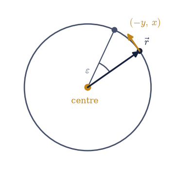
Fig. 120 Rotational symmetry of a central potential: a particle at position \(\vec r\) (radius \(r\) from the force centre, amber) is carried to its image by a small rotation through angle \(\varepsilon\) about the centre, along the constant-\(r\) circle (grey); the rotation generator \((\delta x,\delta y)=(-y,x)\) is tangent to the circle, and because the rotation preserves \(x^2+y^2\) the Lagrangian is invariant, so angular momentum is conserved.#
central potential, dL/dε|0 = 0 ⇒ rotation is a symmetry
✓ the central-potential Lagrangian is rotationally invariant [dL/dε|0 = 0]
True
Exercise 2 — Build the Noether charge from the symmetry#
This is the theorem doing its job: the symmetry produces the conserved quantity. The infinitesimal rotation generator is read off from the flow by differentiating at \(\varepsilon=0\): \((\delta x, \delta y) = \tfrac{\mathrm d}{\mathrm d\varepsilon}(x(\varepsilon), y(\varepsilon))|_0 = (-y, x)\). The rotation leaves \(\mathcal L\) strictly invariant, so \(f=0\), and Noether’s charge Eq. 139 is \(Q = p_x\,\delta x + p_y\,\delta y\) with \(p_x = \partial\mathcal L/\partial v_x\), \(p_y = \partial\mathcal L/\partial v_y\). Nowhere in what follows is angular momentum assumed: whatever that assembly returns, the symmetry put it there.
Write
noether_charge(L, vels, dq, f=0), assembling the conserved charge Eq. 139 from the Lagrangian, the velocity symbols, the generator components \(\delta q_i\) and the optional boundary function: sum \(\partial\mathcal L/\partial v_i \cdot \delta q_i\) over the coordinates, subtract \(f\), and simplify. Write this one yourself — the implementation is the lesson.Take unit mass (\(m=1\)) for the algebra, build \(Q\) for the rotation generator with your
noether_charge, and show it simplifies to \(x\,v_y - y\,v_x\): the angular momentum \(L_z\) Eq. 142, handed to us by the rotational symmetry.
Noether charge of rotation: Q = -v_x*y + v_y*x
Q − (x v_y − y v_x) = 0
✓ the Noether charge of rotational symmetry IS angular momentum [constructed charge Q = -v_x*y + v_y*x]
True
Exercise 3 — Rotational symmetry ⇒ angular momentum (numeric)#
Symbol-level invariance promises conservation along solutions of the equations
of motion. Time to integrate an actual trajectory and watch \(L_z\)
Eq. 142 hold. We reuse the pipeline of §2.1: build the central-potential
Lagrangian in Cartesian coordinates \(x(t), y(t)\) (Cartesian avoids the polar
coordinate singularity at the origin), let euler_lagrange derive the EOM, and
to_numeric + solve_ivp integrate a bound orbit.
Your task. Integrate the orbit with to_numeric + scipy.integrate.solve_ivp
(DOP853, rtol=1e-11, atol=1e-12) on a dense t_eval, compute
\(L_z(t) = m(x\dot y - y\dot x)\) along it, confirm it is conserved, and plot the orbit.
L_z relative drift = 9.45e-11
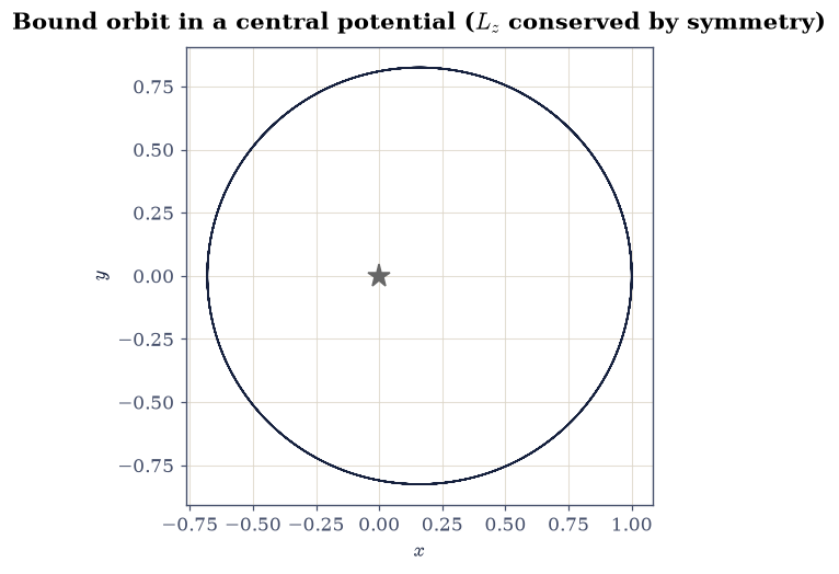
✓ angular momentum conserved under rotational symmetry [max relative drift = 5.09409e-11 (limit 1e-06)]
True
Exercise 4 — Time-translation ⇒ energy (numeric)#
The same trajectory carries a second conservation law. The central-potential Lagrangian has no explicit time dependence, so time-translation \(t \to t + \varepsilon\) is a symmetry and the conserved charge Eq. 140 is the total energy \(E = T + V = \tfrac12 m(\dot x^2 + \dot y^2) - k/r\). (For a Lagrangian of the form \(T - V\) with velocity-independent \(V\), the abstract charge \(\sum_i \dot q_i\,\partial_{\dot q_i}\mathcal L - \mathcal L\) reduces to exactly \(T + V\).)
Your task. Reconstruct \(E(t)\) along the Exercise 3 trajectory
(numpy.hypot for \(r\)) and confirm it is conserved to tight tolerance: a
second, independent symmetry giving a second conserved quantity on the very
same orbit.
E relative drift = 2.09e-10
✓ energy conserved under time-translation symmetry [max relative drift = 1.37805e-10 (limit 1e-06)]
True
Exercise 5 — The contrast: break the symmetry, lose the law#
This is the centrepiece, and it is where the converse earns its keep. We add a single term to the potential, \(V \to V + b\,x\): a uniform force in the \(x\)-direction, as if the orbiting particle felt a constant pull. This term has a preferred direction, so it breaks rotational invariance. But it carries no explicit time dependence, so time-translation invariance survives untouched.
Noether’s theorem then makes a sharp, falsifiable prediction: angular momentum should stop being conserved, while energy should remain conserved. We check it on both fronts: symbolically (the rotational defect is now nonzero) and numerically (integrate the perturbed orbit and watch \(L_z\) come apart while \(E\) stays flat).
Recompute the rotational defect for \(\mathcal L_{\text{broken}} = \tfrac12 m(v_x^2+v_y^2) + k/r - b\,x\) with the
invariance_defectyou wrote in Exercise 1, and confirm it is now nonzero.Integrate the perturbed orbit (same
solve_ivp/DOP853settings as Exercise 3); compute \(L_z(t)\) and \(E(t)\).Make the figure that is the lesson: \(L_z(t)\) for the symmetric orbit (flat) against \(L_z(t)\) for the broken orbit (wildly varying) on one axes, and \(E(t)\) relative drift for both (flat in both) below it.
broken Lagrangian, dL/dε|0 = b*y ⇒ NOT rotationally invariant
broken L_z swings -90.5 → 1.2 (ptp/|L_z(0)| = 101.9)
broken E relative drift = 4.60e-10
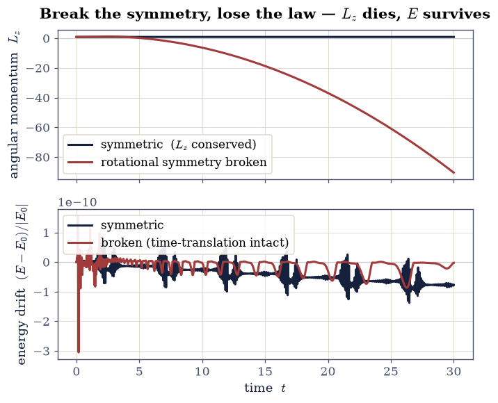
✓ breaking rotational symmetry destroys angular-momentum conservation [L_z varies by 101.9× its initial value]
✓ energy is still conserved (time-translation symmetry intact) [max relative drift = 3.04998e-10 (limit 1e-06)]
True
Exercise 6 — Translational symmetry ⇒ total momentum (worked animation)#
Now a symmetry that mixes particles rather than directions. Two bodies interact only through a potential that depends on their separation, \(V(|\mathbf r_1 - \mathbf r_2|)\), with no external field: here the gravitational \(V = -G m_1 m_2/|\mathbf r_1 - \mathbf r_2|\). Shifting both particles by the same displacement leaves \(|\mathbf r_1 - \mathbf r_2|\) (and hence \(\mathcal L\)) unchanged: the system is translationally invariant. By Eq. 141 the total linear momentum \(\mathbf P = m_1\dot{\mathbf r}_1 + m_2\dot{\mathbf r}_2\) is conserved, which means the centre of mass moves in a straight line at constant velocity no matter how complicated the internal orbit.
This is the worked animation; you build the second in Exercise 7. We give the pair a net drift velocity so the conserved momentum is plainly nonzero: the two bodies wheel around each other while their centre of mass (marked) sails through the frame on a perfectly straight track.
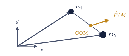
Fig. 121 Translational symmetry of an isolated two-body system: masses \(m_1\) and \(m_2\) with position vectors \(\vec r_1,\vec r_2\) from a fixed origin interact through a potential depending only on their separation \(|\vec r_1-\vec r_2|\) (grey link), so a common shift of both bodies leaves the Lagrangian unchanged; the total momentum is conserved and the centre of mass (COM, amber) moves at constant velocity \(\vec P/M\).#
total |P| relative drift = 2.59e-15
COM speed: start 0.3000, vx drift 7.8e-16
Fig. 122 Animation of two gravitating bodies \(m_1=m_2=1\) given a net drift: the bodies (blue, orange) wheel around each other while their centre of mass (red cross) sails along the dashed straight track at constant velocity, the visible signature of conserved total linear momentum from translational invariance.#
✓ total linear momentum conserved (translational symmetry) [max relative drift = 1.4803e-15 (limit 1e-06)]
True
Notebook summary#
Noether’s theorem made operational: a symbolic test that a transformation leaves the Lagrangian invariant, and the construction of the conserved Noether charge from it.
The canonical pairings confirmed numerically (conserved along
solve_ivptrajectories): rotational symmetry ⇒ angular momentum, time-translation ⇒ energy, spatial translation ⇒ total momentum; and the contrast that breaking the symmetry destroys the conservation law.
Outlook#
The energy/Jacobi distinction. When \(\mathcal L\) is explicitly time-dependent, energy Eq. 140 is no longer conserved, but for a system written in a steadily rotating frame the Jacobi integral \(h = \sum_i \dot q_i\,\partial_{\dot q_i}\mathcal L - \mathcal L\) still is. It is the charge of a different time-translation, and the gap between \(h\) and \(T+V\) is exactly the rotating-frame energy bookkeeping.
Scaling symmetry and the virial theorem. Mechanical similarity (rescaling lengths and times together) is a symmetry of power-law potentials, and it yields the virial relation between average kinetic and potential energies (Landau & Lifshitz §10).
Why continuous? Noether’s theorem needs a continuous symmetry: the charge is built from the generator \(\delta q_i\), which only exists for transformations one can do infinitesimally. Discrete symmetries (parity, time reversal) give powerful selection rules but no conserved Noether charge.
Noether in field theory. Replace “coordinate” by “field” and the very same construction gives conserved currents. In electromagnetism the relevant continuous symmetry is gauge invariance, and the conserved charge is electric charge itself: a thread we pick up in Volume III.