6.26 The Density Matrix, Mixed States, and Decoherence

Elementary Computational Physics

Volume VI — Quantum Mechanics Notebook 6.26

What is the state of half an entangled pair? No single wavefunction will do. The density matrix is the object that describes it — and with it, the difference between a genuine superposition and a mere statistical mixture, the entanglement of a subsystem measured as an entropy, and the way a quantum system loses its coherence to the environment and starts to look classical. It is also the state on which quantum statistical mechanics will later be built.

Level · advanced   •   Est. · 170–210 min

Raymond Amador v1.4.0  ·  2026-07-31  ·  CC BY 4.0 (text) / MIT (code)

Notebook overview

A puzzle has run through this movement: what is the state of one half of an entangled pair? The Bell state (§6.8) and the Bell inequality (§6.25) kept showing single-particle marginals that looked completely random, yet no state vector for a single particle reproduces that. A state vector \(|\psi\rangle\) describes a system we know as well as quantum mechanics allows — a pure state — but two situations escape it: a statistical mixture (we are classically uncertain which pure state we have, like an unpolarized beam) and a subsystem of an entangled whole (where no state vector for the part exists at all). The density operator \(\rho\) handles both.

For a pure state \(\rho=|\psi\rangle\langle\psi|\); for a mixture \(\rho=\sum_i p_i |\psi_i\rangle\langle\psi_i|\). It is Hermitian, positive, and unit-trace, and every prediction follows from it, \(\langle A\rangle=\mathrm{Tr}(\rho A)\). Crucially \(\rho\) distinguishes a coherent superposition from a mixture — the superposition carries nonzero off-diagonal coherences and a definite value in a rotated basis, the mixture does not — a distinction a bare list of probabilities erases. The purity \(\mathrm{Tr}(\rho^2)\) diagnoses which. For a composite system the state of one part is the reduced density matrix \(\rho_A=\mathrm{Tr}_B\rho\), and here the deep fact surfaces: a pure entangled whole has mixed parts. The reduced state of a Bell pair is maximally mixed (purity \(\tfrac12\), von Neumann entropy \(1\) bit) — which is exactly why the marginals of §6.8 and §6.25 were random. That entropy measures the entanglement. Finally decoherence: when a superposition entangles with an environment we then ignore, its coherences decay and it becomes a classical mixture — the mechanism of the quantum-to-classical transition, and the practical adversary of every qubit.

Scope boundary. We develop \(\rho\) for entanglement, mixed states, and decoherence. The same object also carries a thermal weight, \(\rho=e^{-\beta H}/Z\), and is the starting point of quantum statistical mechanics — but the thermal state, partition functions, and the Fermi–Dirac / Bose–Einstein distributions are deferred to Volume VII. Here \(\rho\) is the language of entanglement. Lindblad / open-system dynamics and quantum channels are named as horizons, not developed.

Method specificity. \(\rho=|\psi\rangle\langle\psi|\) via numpy.outer; \(\langle A\rangle=\mathrm{Tr}(\rho A)\) via numpy.trace; the partial trace via numpy.reshape + numpy.trace over the traced indices; the von Neumann entropy from numpy.linalg.eigvalsh; and scipy.linalg.expm for the von Neumann evolution. Entropy is in bits (\(\log_2\)).

Theory in brief

Why a state vector is not enough

\(|\psi\rangle\) describes a pure state — maximal knowledge. But an unpolarized beam (a classical 50/50 mixture of up and down) and one half of an entangled pair cannot be written as any single \(|\psi\rangle\). We need an object for mixtures and subsystems.

(636)\[\text{pure: } |\psi\rangle \qquad\text{vs}\qquad \text{mixture / subsystem: no single } |\psi\rangle \text{ exists.}\]

The density operator

For a pure state \(\rho=|\psi\rangle\langle\psi|\); for a mixture of pure states \(|\psi_i\rangle\) with classical probabilities \(p_i\),

(637)\[\rho = \sum_i p_i\,|\psi_i\rangle\langle\psi_i| , \qquad \rho=\rho^\dagger,\quad \rho\succeq0,\quad \mathrm{Tr}\,\rho=1 ,\]

and every prediction is \(\langle A\rangle=\mathrm{Tr}(\rho A)\) (equal to \(\langle\psi|A|\psi\rangle\) for a pure state); the diagonal entries are outcome probabilities.

Superposition versus mixture

The essential lesson. The pure superposition \((|0\rangle+|1\rangle)/\sqrt2\) and the mixture \(\tfrac12|0\rangle\langle0|+\tfrac12|1\rangle\langle1|\) have the same diagonal (50/50 in the computational basis) but different off-diagonals:

(638)\[\begin{split}\rho_{\text{sup}}=\tfrac12\begin{pmatrix}1&1\\1&1\end{pmatrix},\qquad \rho_{\text{mix}}=\tfrac12\begin{pmatrix}1&0\\0&1\end{pmatrix}.\end{split}\]

The superposition’s off-diagonal coherences make it give a definite result in a rotated basis (\(\langle\sigma_x\rangle=1\)); the mixture stays random (\(\langle\sigma_x\rangle=0\)). They are physically distinct states.

Purity

The purity \(\mathrm{Tr}(\rho^2)\) is \(1\) iff \(\rho\) is pure, and smaller for mixed states, down to \(1/d\) for the maximally mixed state.

(639)\[\mathrm{Tr}(\rho^2) = \frac{1+r^2}{2}\quad(\text{qubit, Bloch length }r): \ 1 \text{ on the Bloch surface},\ \tfrac12 \text{ at the center.}\]

The Bloch sphere of §6.8, now filled in: pure states on the surface, mixed states in the interior.

The reduced density matrix and the partial trace

For a composite system \(AB\), the state of \(A\) alone is the reduced density matrix obtained by the partial trace over \(B\),

(640)\[\rho_A = \mathrm{Tr}_B\,\rho_{AB} = \sum_k \langle k|_B\,\rho_{AB}\,|k\rangle_B ,\]

computed by reshaping to \((d_A,d_B,d_A,d_B)\) and tracing the \(B\) indices. It gives the correct statistics for any measurement on \(A\) alone.

Entanglement makes parts mixed

The deep result. For a Bell state the whole is pure but each part is maximally mixed:

(641)\[|\Phi\rangle=\tfrac1{\sqrt2}(|00\rangle+|11\rangle)\ \text{pure},\qquad \rho_A=\tfrac12 I,\quad S(\rho_A)=-\!\sum_k\lambda_k\log_2\lambda_k = 1\ \text{bit.}\]

A pure entangled state has mixed subsystems — exactly why the single-particle marginals of §6.8 and §6.25 are random. The von Neumann entropy \(S(\rho)\) is \(0\) for a pure state and \(1\) bit for a maximally mixed qubit; for a pure bipartite state \(S(\rho_A)\) is the entanglement entropy.

Decoherence

How the classical world emerges. Let a superposition entangle with an environment that records which state it is in, \((|0\rangle|E_0\rangle+|1\rangle|E_1\rangle)/ \sqrt2\); tracing out the environment leaves a system coherence proportional to the overlap \(\langle E_0|E_1\rangle\):

(642)\[\begin{split}\rho_S = \tfrac12\begin{pmatrix}1&\langle E_1|E_0\rangle\\ \langle E_0|E_1\rangle&1 \end{pmatrix} \xrightarrow{\ \langle E_0|E_1\rangle\to0\ } \tfrac12 I .\end{split}\]

As the environment distinguishes the states, the coherences decay and the pure superposition becomes a classical mixture (purity \(1\to\tfrac12\)) — why macroscopic superpositions are never seen, and why qubits must be isolated.

Evolution of the density matrix

For a closed system, \(\rho(t)=U(t)\rho(0)U^\dagger(t)\), equivalently the von Neumann equation

(643)\[i\hbar\,\frac{\mathrm d\rho}{\mathrm dt} = [H,\rho] ,\]

the density-matrix form of the Schrödinger equation. Under unitary evolution purity is conserved — mixing never arises from closed dynamics, only from tracing out an environment (decoherence) or classical ignorance.

• Reference: Sakurai & Napolitano (§3.4); Nielsen & Chuang [NC10] (density matrices, partial trace, von Neumann entropy); Griffiths [GS18] (mixed states). Cross-reference §6.8 (the Bloch sphere, now filled in; the Bell reduced state), §6.25 (the random Bell marginals, now explained), §6.5 (the Born rule), §6.7 (unitary evolution, now for \(\rho\)), and forward to §6.27 (quantum information) and Volume VII (the thermal density matrix — the deferred home). Named as horizons: Lindblad / open-system dynamics, quantum channels, the thermal state.

---

Setup

The data are the conventions — qubits throughout (subsystem dimension 2), \(\hbar=1\), entropy in bits (\(\log_2\)), and numpy.kron ordering that puts factor \(A\) first — together with the computational-basis kets \(|0\rangle,|1\rangle\) and the Pauli matrices of §6.6, the fixed objects every state and observable below is written in terms of. The instruments are the three meters that read a number off a density matrix once it exists: expectation(rho, A) for \(\langle A\rangle=\mathrm{Tr}(\rho A)\) (numpy.trace), purity(rho) for \(\mathrm{Tr}(\rho^2)\), and von_neumann_entropy(rho) for \(-\sum_k\lambda_k\log_2\lambda_k\) from numpy.linalg.eigvalsh. This notebook’s own machinery is not here: you write the density operator density_matrix in Exercise 1, the partial trace partial_trace in Exercise 4, and the von Neumann evolution evolve_density in Exercise 8. No randomness appears anywhere in this notebook.

The Setup below holds this notebook’s data and instruments — nothing you are asked to build. It is collapsed so the building stays yours; expand it whenever you want the details.

Show code cell source

Hide code cell source

import numpy as np
from scipy.linalg import expm
import matplotlib.pyplot as plt

from ecp import draw, validate

# data: conventions. ℏ=1; qubits throughout (subsystem dimension 2); entropy in bits (log₂);
# numpy.kron(a, b) puts factor A first, so |q_A q_B⟩ is index 2·q_A + q_B.
HBAR = 1.0

# data: the computational basis and the Pauli matrices of §6.6 — the fixed specimens
KET0 = np.array([1.0, 0.0], dtype=complex)
KET1 = np.array([0.0, 1.0], dtype=complex)
SIGMA_X = np.array([[0.0, 1.0], [1.0, 0.0]], dtype=complex)
SIGMA_Y = np.array([[0.0, -1j], [1j, 0.0]], dtype=complex)
SIGMA_Z = np.array([[1.0, 0.0], [0.0, -1.0]], dtype=complex)


# instrument: the reading device, one numpy.trace. Every exercise measures *with* it; the
# Born-rule content behind ⟨A⟩ is the lesson of §6.5, not of this notebook.
def expectation(rho, A):
    r"""Expectation value $\langle A\rangle=\mathrm{Tr}(\rho A)$ (`numpy.trace`)."""
    return float(np.real(np.trace(rho @ A)))


# instrument: a mixedness meter. What the exercises put under test is which states come out
# pure and which mixed, not how Tr(ρ²) is evaluated.
def purity(rho):
    r"""Purity $\mathrm{Tr}(\rho^2)$ {eq}`eq-purity`: 1 for pure, $1/d$ for maximally mixed."""
    return float(np.real(np.trace(rho @ rho)))


# instrument: the second mixedness meter — the 5.x Shannon/von-Neumann entropy formula
# applied to a density matrix's eigenvalues. The lesson is the value it returns for a Bell
# half, not its arithmetic.
def von_neumann_entropy(rho):
    r"""Von Neumann entropy $S=-\sum_k\lambda_k\log_2\lambda_k$ in bits.

    The eigenvalues come from `numpy.linalg.eigvalsh`; zero (and tiny negative,
    round-off) eigenvalues are dropped, since $0\log0=0$.

    Parameters
    ----------
    rho : numpy.ndarray
        A density matrix.

    Returns
    -------
    float
        The entropy in bits.
    """
    lam = np.linalg.eigvalsh(rho)
    lam = lam[lam > 1e-12]
    return float(-np.sum(lam * np.log2(lam)))

Exercise 1 — The density operator and its properties

The object this notebook is named for is built from a state in one line: a pure state \(|\psi\rangle\) gives the outer product \(\rho=|\psi\rangle\langle\psi|\), and a classical mixture of pure states \(|\psi_i\rangle\) held with probabilities \(p_i\) gives the weighted sum \(\rho=\sum_i p_i|\psi_i\rangle\langle\psi_i|\) Eq. 637. The two cases share one constructor because a pure state is just the mixture with a single term. Whatever it is built from, the result must be Hermitian, positive semi-definite, and of unit trace — the three axioms that make its diagonal a legitimate list of outcome probabilities — and it must reproduce the state-vector expectation, \(\mathrm{Tr}(\rho A)=\langle\psi|A|\psi\rangle\), for the pure case. The specimens are the pure state \(|\psi\rangle=\cos(0.6)|0\rangle+ \sin(0.6)|1\rangle\), the mixture \(0.7\,|0\rangle\langle0|+0.3\,|1\rangle\langle1|\), and the observable \(A=\sigma_z\).

1. Write density_matrix(spec), returning \(\rho=|\psi\rangle\langle\psi|\) from a ket via numpy.outer (conjugating the second factor), or \(\sum_i p_i|\psi_i\rangle\langle\psi_i|\) when spec is a list of (p, ket) pairs.

2. Check Hermiticity, positivity (eigenvalues \(\ge0\)), and \(\mathrm{Tr}\,\rho=1\).

3. Confirm \(\langle A\rangle=\mathrm{Tr}(\rho A)\) equals \(\langle\psi|A|\psi\rangle\) for the pure case (numpy.trace, the Setup’s expectation).

4. Note the diagonal entries are outcome probabilities.

Cite Eq. 637.

pure: Hermitian=True, positive=True, Tr=1.000000
mixed: Hermitian=True, positive=True, Tr=1.000000
⟨σz⟩:  Tr(ρA) = 0.362358   ⟨ψ|A|ψ⟩ = 0.362358

Validation 1

The density operator must be Hermitian, positive, and unit-trace, and the trace formula must reproduce the state-vector expectation: \(\mathrm{Tr}(\rho A)=\langle \psi|A|\psi\rangle\).

✓  the density operator is Hermitian, positive, and unit-trace
✓  expectation values are ⟨A⟩ = Tr(ρA)   [got 0.362358 vs expected 0.362358 (rtol=1e-09, atol=1e-09)]

True

Exercise 2 — Superposition versus mixture

A coherent superposition and a statistical mixture can carry the same measurement probabilities in one basis and still be different states, and the difference lives in the off-diagonal entries — the coherences. The superposition \((|0\rangle+|1\rangle)/\sqrt2\) and the 50/50 mixture \(\tfrac12|0\rangle\langle0|+\tfrac12|1\rangle\langle1|\) share the diagonal \((\tfrac12,\tfrac12)\), so a computational-basis measurement cannot tell them apart; their off-diagonals differ Eq. 638, and that difference is physical. It shows up as the purity \(\mathrm{Tr}(\rho^2)\), \(1\) against \(\tfrac12\) Eq. 639, and as a measurement along \(x\): the superposition is an eigenstate of \(\sigma_x\) and answers with a definite \(\langle\sigma_x\rangle=1\), while the mixture stays random at \(0\).

1. Build \(\rho\) for both states with the density_matrix you wrote in Exercise 1: the superposition \((|0\rangle+|1\rangle)/\sqrt2\) from its ket, and the 50/50 mixture \(\tfrac12|0\rangle\langle0|+\tfrac12|1\rangle\langle1|\) from its (p, ket) list.

2. Compare their matrices: same diagonal, different off-diagonal.

3. Compute the purity of each (\(1\) vs \(\tfrac12\)).

4. Measure \(\langle\sigma_x\rangle\): definite (\(1\)) for the superposition, random (\(0\)) for the mixture — a measurable difference.

Cite Eq. 638, Eq. 639.

superposition ρ:
 [[0.5 0.5]
 [0.5 0.5]]
mixture ρ:
 [[0.5 0. ]
 [0.  0.5]]
purity:  superposition = 1.000   mixture = 0.500
⟨σx⟩:    superposition = 1.000   mixture = 0.000

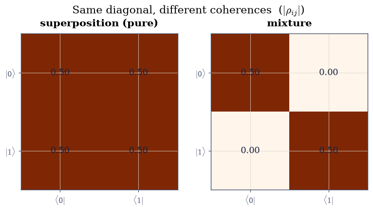
Fig. 598 Coherence is the difference. The coherent superposition \((|0\rangle+|1\rangle)/\sqrt2\) (left) and the 50/50 statistical mixture (right) have identical diagonals — both give 50/50 outcomes in the computational basis — but the superposition carries nonzero off-diagonal coherences (the bright corners) that the mixture lacks. Those coherences are physical: measured along \(x\) the superposition gives a definite \(\langle\sigma_x\rangle=1\) while the mixture stays random at \(0\). A bare list of probabilities would erase the distinction; the density matrix keeps it.

Validation 2

The superposition is pure (purity \(1\), coherences present) and the mixture is mixed (purity \(\tfrac12\)); they differ measurably in \(\langle\sigma_x\rangle\).

✓  a superposition is pure (coherences present) and a 50/50 mixture is mixed   [max|Δ| = 4.44089e-16 (rtol=1e-09, atol=1e-09)]
✓  the superposition gives ⟨σx⟩=1 (definite) while the mixture gives 0 (random)

True

Exercise 3 — Purity and the Bloch ball

The Bloch sphere of §6.8 carried pure states only, on its surface. The density matrix fills it in. Any qubit state whatsoever is \(\rho=\tfrac12(I+\mathbf r\cdot\boldsymbol\sigma)\) for a real Bloch vector \(\mathbf r\) with \(|\mathbf r|\le1\): the sphere becomes a ball, whose interior is exactly the mixed states. The purity is a function of the radius alone, \(\mathrm{Tr}(\rho^2)=(1+r^2)/2\) Eq. 639, so it reads \(1\) on the surface (\(r=1\), pure), falls through the interior, and bottoms out at \(\tfrac12\) at the centre (\(r=0\)), which is the maximally mixed state \(\tfrac12 I\). The specimens are the eleven states along the \(z\) axis, \(\mathbf r=(0,0,r)\) for \(r\) on numpy.linspace(0, 1, 11).

1. Write bloch_density(r_vec), returning \(\rho=\tfrac12(I+\mathbf r\cdot \boldsymbol\sigma)\) for a Bloch vector \(\mathbf r=(x,y,z)\).

2. Compute the purity (the Setup’s purity) as a function of the Bloch length \(r=|\mathbf r|\).

3. Show purity \(=1\) on the surface (\(r=1\), pure) and \(=\tfrac12\) at the center (\(r=0\), maximally mixed).

4. Confirm the closed form \(\mathrm{Tr}(\rho^2)=(1+r^2)/2\).

Cite Eq. 639.

purity vs Bloch length r:
  r=0.0: purity=0.5000  (1+r²)/2=0.5000
  r=0.2: purity=0.5200  (1+r²)/2=0.5200
  r=0.4: purity=0.5800  (1+r²)/2=0.5800
  r=0.6: purity=0.6800  (1+r²)/2=0.6800
  r=0.8: purity=0.8200  (1+r²)/2=0.8200
  r=1.0: purity=1.0000  (1+r²)/2=1.0000

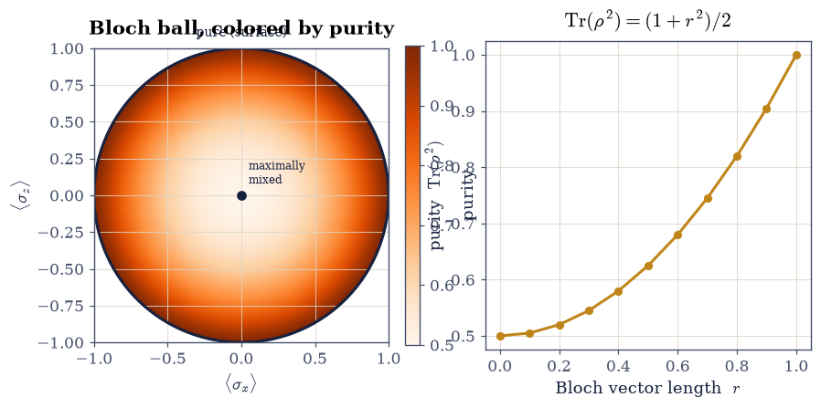
Fig. 599 The Bloch sphere, filled in. Left: a cross-section of the Bloch ball colored by purity — pure states live on the surface (\(r=1\), purity \(1\)), mixed states fill the interior, and the center (\(r=0\)) is the maximally mixed state (purity \(\tfrac12\)). This is the Bloch sphere of §6.8 with mixedness as depth. Right: the purity \(\mathrm{Tr}(\rho^2)=(1+r^2)/2\) rises smoothly from \(\tfrac12\) at the center to \(1\) at the surface. A density matrix is a point in the ball, not just on it.

Validation 3

The qubit purity must follow \((1+r^2)/2\): \(\tfrac12\) at the center (maximally mixed) and \(1\) on the Bloch surface (pure).

✓  qubit purity is (1+r²)/2 — pure on the Bloch surface, maximally mixed at the center   [max|Δ| = 1.11022e-16 (rtol=1e-09, atol=1e-09)]

True

Exercise 4 — The reduced density matrix

Asking what state subsystem \(A\) is in, when only the joint \(\rho_{AB}\) is known, is answered by the partial trace over \(B\), \(\rho_A=\mathrm{Tr}_B\,\rho_{AB}=\sum_k\langle k|_B\, \rho_{AB}\,|k\rangle_B\) Eq. 640. Numerically it is an index contraction: a \(4\times4\) joint matrix carries a hidden four-index structure \(\rho_{(a b),(a'b')}\), so reshaping it to \((d_A,d_B,d_A,d_B)\) exposes the four slots and summing over the matching pair of \(B\) slots — axes \(1\) and \(3\) of the reshaped array — discards \(B\). Getting that pair right is the whole of it: contract axes \(0\) and \(2\) instead and one gets \(\rho_B\), the other subsystem. What certifies the result is that \(\rho_A\) is itself a legitimate density matrix and that it gives the correct statistics for any measurement on \(A\) alone, so that \(\mathrm{Tr}(\rho_A\,\sigma_z)\) agrees with the joint answer \(\mathrm{Tr}(\rho_{AB}\,\sigma_z\otimes I)\). The specimen is the product state \(|\psi\rangle_A\otimes|\phi\rangle_B\) with \(|\psi\rangle=\cos(0.5)|0\rangle+\sin(0.5)|1\rangle\) and \(|\phi\rangle=\cos(1.1)|0\rangle+\sin(1.1)|1\rangle\), whose \(\rho_A\) is known in advance: a product state has an unentangled, and therefore pure, part.

1. Write partial_trace(rho, keep, dims), returning the reduced density matrix of the kept subsystem by numpy.reshape to \((d_A,d_B,d_A,d_B)\) followed by numpy.trace over the traced pair of axes (axis1=1, axis2=3 to keep \(A\), axis1=0, axis2=2 to keep \(B\)). Write this one yourself — the implementation is the lesson.

2. Build the joint \(\rho_{AB}\) for the product state \(|\psi\rangle_A\otimes|\phi\rangle_B\) (numpy.kron, then the density_matrix of Exercise 1) and reduce it with keep=0.

3. Verify \(\rho_A\) is a valid density matrix (Hermitian, positive, unit-trace).

4. Confirm \(\mathrm{Tr}(\rho_A\,\sigma_z)=\mathrm{Tr}(\rho_{AB}\,\sigma_z\otimes I)\) — the reduced state gives the right local statistics.

Cite Eq. 640.

reduced ρ_A:
 [[0.77  0.421]
 [0.421 0.23 ]]
valid: Tr=1.0000, positive=True
⟨σz⟩ on A:  from ρ_A = 0.540302   from ρ_AB (σz⊗I) = 0.540302

Validation 4

The partial trace must yield a valid density matrix for \(A\) that reproduces local expectation values: \(\mathrm{Tr}(\rho_A\,\sigma_z)=\mathrm{Tr}(\rho_{AB}\,\sigma_z \otimes I)\).

✓  the reduced density matrix ρ_A = Tr_B ρ reproduces local expectation values   [got 0.540302 vs expected 0.540302 (rtol=1e-09, atol=1e-09)]
✓  the partial trace yields a valid density matrix (positive, unit-trace)

True

Exercise 5 — A pure whole with mixed parts: entanglement entropy

Here the formalism pays for itself. The Bell state \((|00\rangle+|11\rangle)/\sqrt2\) is a pure state of the pair: we know it as completely as quantum mechanics permits, and its purity is \(1\). Yet reducing it to either half leaves the maximally mixed \(\rho_A=\tfrac12 I\) Eq. 641. Perfect knowledge of the whole, none whatever of the part — an inversion with no classical counterpart, and it is what entanglement is in density-matrix language. The von Neumann entropy \(S(\rho)=-\sum_k\lambda_k\log_2\lambda_k\) over the eigenvalues puts a number on it: \(0\) for a pure state, and for a maximally mixed qubit a full bit, the same one bit of ignorance as a fair coin. For a pure bipartite whole that number is the entanglement entropy. It also closes an old account: the single-particle marginals of §6.8 and §6.25 looked random because the reduced state of a Bell half genuinely is.

1. Confirm the Bell state \((|00\rangle+|11\rangle)/\sqrt2\) has purity \(1\) (a pure whole).

2. Reduce it with your Exercise 4 partial_trace and show \(\rho_A\) is maximally mixed (\(\rho_A=\tfrac12 I\), purity \(\tfrac12\)).

3. Compute \(S(\rho_A)=-\mathrm{Tr}(\rho_A\log_2\rho_A)=1\) bit.

4. Connect to §6.8 / §6.25: tracing out the partner leaves no coherence, so each particle alone looks random.

Cite Eq. 641.

Bell whole:  purity = 1.0000  (pure)
reduced ρ_A:
 [[0.5 0. ]
 [0.  0.5]]
ρ_A:  purity = 0.5000   S(ρ_A) = 1.0000 bit
→ maximally mixed: this is WHY the single-particle marginals of §6.8/§6.25 are random

Validation 5

A pure Bell state must have a maximally mixed reduced state: purity \(\tfrac12\) and von Neumann entropy \(1\) bit.

✓  a pure Bell state has a maximally mixed reduced state, S = 1 bit   [max|Δ| = 2.22045e-16 (rtol=1e-06, atol=1e-09)]

True

Exercise 6 — Entanglement across a family

Entanglement is not a yes-or-no property, and the one-parameter family \(|\psi(t)\rangle=\cos t\,|00\rangle+\sin t\,|11\rangle\) shows why: it passes continuously from the product state \(|00\rangle\) at \(t=0\), through the Bell state at \(t=\pi/4\), to the product state \(|11\rangle\) at \(t=\pi/2\). Every member is pure as a whole, so any entropy found in a half cannot be classical ignorance about the pair. The reduced state’s entropy \(S(\rho_A)\) therefore measures the entanglement and nothing else, rising from \(0\) at the product ends to a full bit at the Bell point Eq. 641, while the reduced purity mirrors it downward from \(1\) to \(\tfrac12\). Maximal entanglement is exactly maximal mixedness of the part.

1. Build the family \(\cos t\,|00\rangle+\sin t\,|11\rangle\) on numpy.linspace(0, numpy.pi/2, 200) with the density_matrix of Exercise 1.

2. For each \(t\) compute \(\rho_A\) with your Exercise 4 partial_trace and its entropy \(S(\rho_A)\) (the Setup’s von_neumann_entropy).

3. Show \(S\) runs from \(0\) at \(t=0\) (product state) to \(1\) bit at \(t=\pi/4\) (Bell).

4. Note \(S(\rho_A)\) is the entanglement measure — maximal exactly when the state is maximally entangled.

Cite Eq. 641.

S(ρ_A):  t=0 → -0.0000   t=π/4 → 1.0000
maximally entangled at t=π/4; product at t=0, π/2

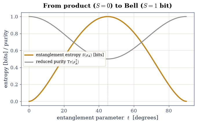
Fig. 600 Entanglement, continuously tuned. For the family \(\cos t\,|00\rangle+\sin t\,|11\rangle\), the entanglement entropy \(S(\rho_A)\) (amber) climbs from \(0\) at the product states (\(t=0,\pi/2\)) to a full bit at the Bell state (\(t=\pi/4\)); the reduced purity (grey) mirrors it, dropping from \(1\) to \(\tfrac12\). The more entangled the whole, the more mixed — and higher-entropy — each part. The entropy of a subsystem is the amount of entanglement.

Validation 6

The entanglement entropy must run from \(0\) (product state, \(t=0\)) to \(1\) bit (Bell state, \(t=\pi/4\)).

✓  the entanglement entropy runs from 0 (product) to 1 bit (Bell)   [max|Δ| = 0 (rtol=1e-06, atol=1e-06)]

True

Exercise 7 — Decoherence

Nothing isolates a real system perfectly, and the previous exercises supply the consequence. Let a superposition interact with an environment that keeps a record of which branch it is in, so that system and environment end in the entangled state \((|0\rangle|E_0\rangle+|1\rangle|E_1\rangle)/\sqrt2\). We do not track the environment, so the state we can speak about is the reduced one, and tracing out the environment leaves a system coherence proportional to the overlap \(\langle E_0|E_1\rangle\) Eq. 642. A perfect record (\(\langle E_0|E_1\rangle=0\), orthogonal environment states) erases the coherence entirely and leaves \(\tfrac12 I\): the pure superposition has become the classical mixture of Exercise 2, with the same diagonal and no interference left. Nothing acted on the system’s outcome statistics in the computational basis; what was lost was the phase relation, to a partner we stopped following. The overlap is swept with the environment states \(|E_0\rangle=(1,0)\) and \(|E_1\rangle=(c,\sqrt{1-c^2})\), so that \(\langle E_0|E_1\rangle=c\), for \(c\) running from \(1\) to \(0\) over numpy.linspace(1, 0, 200).

1. Build the joint system–environment state \((|0\rangle|E_0\rangle+|1\rangle|E_1\rangle)/\sqrt2\) at each \(c\) (numpy.kron, then the density_matrix of Exercise 1).

2. Trace out the environment with your Exercise 4 partial_trace (keep=0).

3. Show the system’s off-diagonal coherence \(|\rho_{01}|\) is proportional to the overlap \(\langle E_0|E_1\rangle=c\).

4. As \(\langle E_0|E_1\rangle\to0\) (the environment distinguishes the states), watch the coherence vanish and the purity drop to \(\tfrac12\) — superposition into mixture.

Cite Eq. 642.

⟨E0|E1⟩ = 1 → 0:  coherence 0.500 → 0.000,  purity 1.000 → 0.500
the pure superposition (purity 1) decoheres into the classical mixture (purity ½)

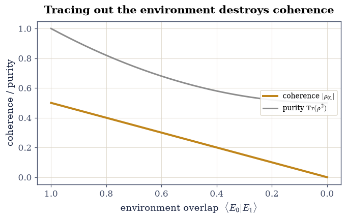
Fig. 601 Decoherence is bookkeeping about a partner you stopped following. As an environment increasingly distinguishes the two branches of a superposition — the overlap \(\langle E_0|E_1\rangle\) falling from \(1\) to \(0\) — the system’s off-diagonal coherence (amber) decays to zero and its purity (grey) drops from \(1\) to \(\tfrac12\). The pure superposition has become a classical mixture, with the same diagonal probabilities but no interference. Nothing changed the outcome statistics in the computational basis; what was lost is the coherence, and with it every quantum signature. This is why macroscopic superpositions are never seen and why qubits must be isolated.

Validation 7

As the environment overlap goes to zero, the system off-diagonal coherence must decay to \(0\) and the purity drop to \(\tfrac12\): tracing out an entangled environment decoheres a superposition into a mixture.

✓  tracing out an entangled environment decoheres a superposition (off-diagonal 0.5→0, purity 1→½) into a classical mixture

True

Exercise 8 — The von Neumann equation and conservation of purity (student)

A state vector evolves by \(|\psi(t)\rangle=U(t)|\psi(0)\rangle\) with \(U(t)=e^{-iHt/\hbar}\) (§6.7); a density matrix, being built from a ket and a bra, picks up the propagator on both sides, \(\rho(t)=U(t)\rho(0)U^\dagger(t)\). Differentiating that sandwich gives the von Neumann equation \(i\hbar\,\mathrm d\rho/\mathrm dt=[H,\rho]\) Eq. 643, the density-matrix form of the Schrödinger equation. It has a consequence worth isolating: since \(U\) is unitary, \(\mathrm{Tr}(\rho^2)\) is invariant, so a pure state evolving under a closed Hamiltonian stays pure forever. Mixing is never manufactured by the dynamics. It arrives only from outside, by tracing out an environment as in Exercise 7 — which is the precise sense in which decoherence is not a force but a loss of bookkeeping. The specimen is the Hamiltonian \(H=0.5\,\sigma_x+0.3\,\sigma_z\) acting on the pure initial state \(\rho(0)=|\chi\rangle\langle\chi|\) with \(|\chi\rangle=(|0\rangle+i|1\rangle)/\sqrt2\), sampled on numpy.linspace(0, 6, 120); the derivative is taken at \(t_0=0.7\) with a centred step \(\mathrm dt=10^{-6}\).

1. Write evolve_density(rho, H, t), returning \(U\rho U^\dagger\) with \(U=e^{-iHt/\hbar}\) from scipy.linalg.expm (not numpy.exp), and evolve \(\rho(0)\) across the time grid.

2. Confirm the von Neumann equation \(i\hbar\,\mathrm d\rho/\mathrm dt=[H,\rho]\) numerically (finite-difference the evolved \(\rho\) against the commutator).

3. Show the purity stays constant — a pure state stays pure.

4. Contrast with decoherence (Ex. 7), where tracing out an environment does reduce purity. Closed dynamics never mixes; only the environment does.

Cite Eq. 643.

purity under unitary evolution: min=1.000000, max=1.000000 (constant)
von Neumann residual max|iℏ dρ/dt − [H,ρ]| = 5.18e-11

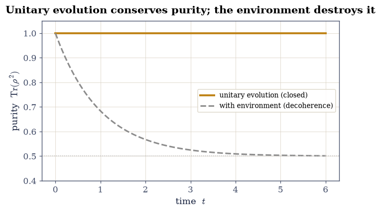
Fig. 602 Closed dynamics never mixes. Under unitary (von Neumann) evolution the purity of a pure state stays pinned at \(1\) (amber) — the state rotates around the Bloch sphere but never leaves the surface, and the von Neumann equation \(i\hbar\,\dot\rho=[H,\rho]\) holds to a part in \(10^{10}\). Mixing can only come from outside the closed system: tracing out an environment (grey, the decoherence of Exercise 7) drives the purity down toward \(\tfrac12\). A qubit left alone stays coherent forever; a qubit watched by its surroundings does not.

Validation 8

Unitary evolution must conserve purity (a pure state stays pure) and satisfy the von Neumann equation; mixing requires an environment, not closed dynamics.

✓  unitary (von Neumann) evolution conserves purity; mixing requires an environment   [max|Δ| = 1.44329e-15 (rtol=1e-06, atol=1e-09)]
✓  the evolved ρ satisfies the von Neumann equation iℏ dρ/dt = [H,ρ]

True

Exercise 9 — (Synthesis) The state, honestly described

The wavefunction was always a best-case description — the state of a system we know as well as nature permits. The density matrix is the honest generalization: it describes what we actually have, whether that is a mixture we are classically uncertain about or a fragment of an entangled whole whose partner we cannot see. It draws the sharp line between a superposition and a mixture that a list of probabilities would erase; it measures entanglement as the entropy of a part; and it shows how a quantum system, by leaking its coherence into an environment it no longer tracks, comes to look classical.

That last point deserves the emphasis this movement has been building toward. The off-diagonal elements of the density matrix are where quantum mechanics lives: keep them and you have interference, coherence, a working qubit; lose them to the environment and you have an ordinary classical alternative. Decoherence is not mysterious — it is bookkeeping about a partner you stopped following. And it closed the loop on the whole movement: the random single-particle marginals of the Bell state (§6.8) and the Bell test (§6.25) are now explained exactly, as the maximally mixed reduced state of a pure entangled whole.

The same object, carrying a thermal weight \(e^{-\beta H}\), will later be the starting point of quantum statistical mechanics — but that is Volume VII. Here it has told us what the entangled states of this movement are truly made of. The final notebook, an optional capstone (§6.27), takes these ideas — mixed states, entropy, entanglement — into the language of quantum information.

Notebook summary

• The density operator Eq. 637: \(\rho=|\psi\rangle\langle \psi|\) (numpy.outer) or \(\sum_i p_i|\psi_i\rangle\langle\psi_i|\); Hermitian, positive, unit-trace, with \(\langle A\rangle=\mathrm{Tr}(\rho A)\).

• Superposition vs mixture Eq. 638: same diagonal, different coherences; purity \(1\) vs \(\tfrac12\); \(\langle\sigma_x\rangle\) \(1\) vs \(0\).

• Purity Eq. 639: \(\mathrm{Tr}(\rho^2)=(1+r^2)/2\) — the Bloch sphere filled in, pure on the surface and maximally mixed at the center.

• The partial trace Eq. 640: \(\rho_A=\mathrm{Tr}_B\rho\) (numpy.reshape + numpy.trace) gives correct local statistics.

• Entanglement = mixed parts Eq. 641: a pure Bell state has \(\rho_A=\tfrac12 I\), \(S=1\) bit — why §6.8/§6.25 marginals are random; \(S(\rho_A)\) runs \(0\to1\) bit across the entanglement family.

• Decoherence Eq. 642: tracing out an environment sends the coherence \(\to0\) and purity \(\to\tfrac12\) — superposition into mixture.

• Von Neumann evolution Eq. 643: \(i\hbar\dot\rho=[H,\rho]\); closed dynamics conserves purity (scipy.linalg.expm), so mixing needs an environment.

Scope reminder. The thermal density matrix \(\rho=e^{-\beta H}/Z\) and quantum statistical mechanics are built on exactly this object — but that is Volume VII. Here \(\rho\) served entanglement, mixed states, and decoherence.

Outlook

• Quantum information (§6.27, optional capstone): density matrices, entropy, and quantum channels.

• The thermal density matrix \(\rho=e^{-\beta H}/Z\) and quantum statistical mechanics — the deferred home (Volume VII).

• Open quantum systems and Lindblad dynamics; the full theory of decoherence (horizons).

• Quantum error correction and why decoherence is the central obstacle to quantum computing (a horizon).

• Cross-reference §6.8 (Bloch sphere, Bell reduced state), §6.25 (Bell marginals), §6.5 (Born rule), §6.7 (unitary evolution), forward to §6.27, Volume VII.

References

[GS18]

David J. Griffiths and Darrell F. Schroeter. Introduction to Quantum Mechanics. Cambridge University Press, 3 edition, 2018.

[NC10]

Michael A. Nielsen and Isaac L. Chuang. Quantum Computation and Quantum Information. Cambridge University Press, 10th anniversary edition, 2010.

Take this notebook with you

Use the download button (↓) in the toolbar above to save this notebook and run it yourself. The published notebooks ship without worked solutions; if you would like the reference solutions — to teach from or to check your own work — get in touch: hello@ramador.me.