7.18 Quantum Paramagnets: The Brillouin Function and the Refrigerator

Elementary Computational Physics

Volume VII — Quantum Statistical Mechanics Notebook 7.18

N spins in a field is the simplest magnet there is, and it contains multitudes: set J to one-half and this volume's warm qubit reappears; send J to infinity and the classical paramagnet emerges as a limit; expand at small field and Curie's law hands you the square of the angular momentum on a susceptibility slope. One 1952 experiment lays three real salts exactly on the predicted curves — and the entropy of the same spin bath, released by switching off a magnet, is the refrigerator that carried physics below one kelvin.

Level · advanced   •   Est. · 185–225 min

Raymond Amador v1.4.0  ·  2026-07-31  ·  CC BY 4.0 (text) / MIT (code)

Notebook overview

Movement V opens with the simplest interaction-free magnet there is — \(N\) independent spins \(J\) in a field — and finds in it three limits of the volume, one great experiment, and the refrigerator on which low-temperature physics was built. The model is the multiplet of §6.18 put to work at temperature: levels \(E_m = -g\mu_BBm\), a geometric sum for the partition function, and one function for the magnetization: the Brillouin function \(B_J(x)\). Its three limits are three cross-references made good. At \(J = 1/2\) it is \(\tanh x\), identically (verified below to \(2\times10^{-15}\)): the warm qubit of §7.4 was a Brillouin paramagnet all along, the bottom rung of a ladder. At \(J \to \infty\) it becomes the classical Langevin function \(\coth x - 1/x\), converging as \(\sim 1/J\): the paramagnet of pre-quantum physics is the infinite-spin limit, one more classical result derived as a limit, and the tally that already holds \(h\), \(\sigma\), and \(N!\) gains a fourth entry. And at small \(x\) it gives Curie’s law with its \(J(J+1)\): the thermodynamic magnet measures the square of the angular momentum: the eigenvalue of §6.18, extracted from a susceptibility slope on a lab bench.

A dramatic numerical trap sits exactly where the physics lives. \(B_J\) is a difference of two \(\coth\) terms that each diverge as \(1/x\), and the difference is \(O(x)\): naive evaluation holds eight digits at \(x = 10^{-4}\) and keeps zero correct digits at \(x = 10^{-8}\): total cancellation (the return is pure round-off — 0.0 or a stray last bit of \(1/x\), depending on the platform), in precisely the small-\(x\) regime where Curie constants are measured. The series switch is mandatory, and the general rule (differences of divergent terms are never evaluated naively) joins expm1 in the course’s standing kit. The data jewel is Henry 1952: the magnetization of three paramagnetic salts — Cr³⁺ (\(S = 3/2\)), Fe³⁺ (\(5/2\)), Gd³⁺ (\(7/2\)) — measured between 1.3 and 4.2 K up to 5 T, falling on pure Brillouin curves as functions of \(B/T\) alone and saturating at \(3\), \(5\), \(7\,\mu_B\); the effective-moment pipeline \(p_{\text{eff}} = g\sqrt{J(J+1)}\) then reads atomic angular momenta off bulk susceptibilities, with the quenching honesty attached (why \(S\) rather than \(J\): crystal fields).

The centerpiece is the entropy and the machine built on it. For the ideal paramagnet \(S\) depends on \(B\) and \(T\) only through \(B/T\) (verified to all digits, because the partition function contains no other scale), so an adiabat is \(B/T = \text{const}\), and adiabatic demagnetization cools by pure bookkeeping: magnetize isothermally (dump the spin entropy to a helium bath), then demagnetize adiabatically and ride \(B/T\) down, \(T_f = T_i\,B_f/B_i\), verified by exact solve to 50.00 mK. The honest floor: internal fields \(b \sim 10\) mT keep the effective field finite and floor the cycle near \(T_i\,b/B_i \approx 10\) mK, which is also the third law enforcing itself. Giauque reached 0.25 K this way in 1933 (Nobel 1949); nuclear moments extend the trick to microkelvin; and adiabatic demagnetization refrigerators fly on X-ray satellites today. The meta-point is worth reading aloud: this notebook’s refrigerator made the volume’s own data possible; the sub-3-K calorimetry of §7.10 and every \(\theta_D\) in §7.16 sit downstream of Giauque’s salt pill. The closing contrast draws the susceptibility of §7.10 as a diagnostic (Curie \(1/T\) against Pauli-flat on one \(\chi T\) panel), and the Curie–Weiss \(\theta\) that bends real data is the first fingerprint of spin–spin interactions: the independence assumption’s expiry date, and the opening of §7.19.

Conventions (this notebook). Two reduced variables, kept scrupulously apart: \(y = g\mu_BB/k_BT\) is the partition function’s natural variable, and \(x = Jy\) is the Brillouin function’s argument — a silent \(J\)-factor slip rescales every curve, so the convention is stated here once and audited where used. Entropies and heat capacities are per spin; magnetizations per ion in units of \(\mu_B\) (Henry’s units). The quenched \(3d\) salts take \(g = 2\) with spin-only \(S\) (the quenching note in Exercise 4). All large-\(y\) thermodynamics uses ground-shifted weights \(e^{y(m-J)}\) — the stabilization discipline of §7.17, re-applied — and the small-\(x\) Brillouin branch switches to its series at the stated threshold \(x = 2\times10^{-3}\), justified by branch-matching. Demagnetization solves use scipy.optimize.brentq on the exact entropy curves, with the below-floor no-solution case handled explicitly.

How to read the checks. Each exercise closes with a validate call against an independent fact: the geometric-sum identity at ten digits; \(\tanh\) recovered at machine precision; the Langevin approach and the Curie slope; the naive form’s total digit loss against the repaired branch; the theory values at Henry’s \(B/T\) frontier; the \(p_{\text{eff}}\) pipeline run as a fit; the entropy’s single-variable property from the \((B, T)\) interface; the 50 mK and 10 mK solves; the \(\chi T\) decompositions. A ✓ is strong evidence; a ✗ is a prompt to locate the discrepancy.

Scope. Crystal-field theory and rare-earth (\(L \ne 0\), full Landé) magnetism, Curie–Weiss ordering and mean-field magnetism, nuclear demagnetization, and satellite ADRs are named horizons. See Henry, Phys. Rev. 88, 559 (1952); Giauque & MacDougall 1933; Kittel (Ch. 11); Ashcroft & Mermin (Ch. 31); Pathria & Beale. Cross-reference §6.18 (the moment, in full), §7.4 (\(\tanh\): the bottom rung), §7.10 (the itinerant contrast), §7.15 (the same levels, inverted), §7.17 (the ground-shift discipline), §5.10 (the classical chain awaiting its quantum counterpart), and forward to §7.19.

Theory in brief

Spin J at temperature

The multiplet of §6.18 in a field along \(z\): \(2J+1\) levels \(E_m = -g\mu_BBm\), \(m = -J,\dots,J\). The single-spin partition function is a geometric sum with ratio \(e^{y}\) (\(y = g\mu_BB/k_BT\)):

(794)\[z = \sum_{m=-J}^{J} e^{ym} = \frac{\sinh\!\big[(2J{+}1)\,y/2\big]}{\sinh\!\big[y/2\big]}, \qquad M = Ng\mu_BJ\,B_J(x), \quad x = Jy,\]

with the Brillouin function \(B_J(x) = \frac{2J+1}{2J}\coth\frac{(2J+1)x}{2J} - \frac{1}{2J}\coth\frac{x}{2J}\). The two variables deserve their own sentence: \(y\) is the level-spacing scale the partition function knows; \(x = Jy\) is the total-moment scale the magnetization curve collapses in; mixing them rescales every plot by \(J\).

Three limits, three cross-references

Each limit follows from the definition of \(B_J\) by elementary means: setting \(J = 1/2\) collapses the two \(\coth\) terms into a single \(\tanh\), while \(J \to \infty\) and \(x \to 0\) are Taylor expansions (Kittel, Ch. 11, works them all). What matters here is where each limit lands in the course:

(795)\[B_{1/2}(x) = \tanh x, \qquad B_{J\to\infty}(x) \to L(x) = \coth x - \frac1x, \qquad B_J(x\to0) \to \frac{(J+1)x}{3J} \;\Rightarrow\; \chi = \frac{Ng^2\mu_B^2\,J(J+1)}{3k_BT}.\]

\(J = 1/2\) is the warm qubit of §7.4, identically: the ladder’s bottom rung. \(J \to \infty\) is the classical paramagnet: Langevin’s 1905 function, derived a century before as an integral over classical dipole orientations, emerges here as the infinite-spin limit at \(\sim 1/J\); the tally of classical results demoted to limits (\(h\) in §7.5, \(\sigma\) in §7.6, \(N!\) in §7.8) gains its fourth entry. And the small-\(x\) slope carries \(J(J+1)\): Curie’s law measures the square of the angular momentum, never the vector: the eigenvalue structure of §6.18 showing up as the slope of \(1/\chi\) against \(T\). At the other end \(B_J \to 1\): saturation at \(gJ\mu_B\) per ion.

The cancellation trap

Numerical trouble hides in plain sight in the definition of \(B_J\): annotate each \(\coth\) term with its small-\(x\) behavior and the subtraction announces itself:

(796)\[B_J(x) = \underbrace{\tfrac{2J+1}{2J}\coth\tfrac{(2J+1)x}{2J}}_{\sim 1/x} \; - \; \underbrace{\tfrac{1}{2J}\coth\tfrac{x}{2J}}_{\sim 1/x} \;=\; O(x).\]

Both terms diverge as \(1/x\); the physics is their tiny difference. In floating point the physics drowns beneath the \(1/x\) terms’ rounding floor once \(x\) is small enough — the naive form holds eight digits at \(x = 10^{-4}\) and keeps zero correct digits at \(x = 10^{-8}\) (demonstrated below: the return is pure round-off, exactly 0.0 or a stray last bit of the \(1/x\) terms depending on the platform’s tanh), and \(x \sim 10^{-8}\) is a perfectly ordinary Curie-regime value (\(\mu\)T fields at kelvin temperatures). The mandatory fix is a series branch, \((J+1)x/3J - [(2J+1)^4-1]x^3/45(2J)^4\), switched in by numpy.where below a threshold justified by matching the two branches. The standing rule: differences of divergent terms are never evaluated naively.

Henry 1952: three salts, three curves (data)

The magnetization law above contains only two material inputs, \(g\) and \(J\), so dividing out the ion count and the Bohr magneton leaves a prediction with nothing left to tune:

(797)\[\frac{M}{N\mu_B} = gJ\,B_J\!\left(\frac{g\mu_BJB}{k_BT}\right) \quad\text{— one curve per ion, in } B/T \text{ alone.}\]

Henry measured the magnetization of chromium potassium alum (Cr³⁺, \(S = 3/2\)), iron ammonium alum (Fe³⁺, \(5/2\)), and gadolinium sulfate octahydrate (Gd³⁺, \(7/2\)) between 1.3 and 4.2 K in fields to 5 T, and the points fall on pure Brillouin curves: saturation at \(3\), \(5\), \(7\,\mu_B\) per ion, and (the single-variable prediction made visible) data taken at four different temperatures collapsing onto one curve per ion when plotted against \(B/T\). At Henry’s frontier \(B/T = 3.85\) T/K the theory reads \(2.989/4.989/6.989\,\mu_B\): saturation reached to a percent. The honesty in three sentences: these are spin-only values with \(g \approx 2\) because the crystal field quenches the \(3d\) orbital moment; Gd³⁺ is the clean case because its half-filled shell has \(L = 0\); crystal-field theory, and the rare-earth ions where the full Landé \(g_J\) and \(J\) survive, are the outward horizon. The effective-moment pipeline completes the loop: \(p_{\text{eff}} = g\sqrt{J(J+1)} = 3.873/5.916/7.937\) against the measured \(\sim3.8/5.9/8.0\) — atomic structure read off a bulk \(\chi T\).

The entropy of a spin bath

The entropy follows from the geometric-sum partition function by one derivative of the free energy, \(S = -\partial F/\partial T\) with \(F = -k_BT\ln z\) per spin; written in the reduced variable, the result is

(798)\[\frac{S}{k_B} = \ln z - y\,\langle m\rangle, \qquad S = S(y)\ \text{only}, \qquad S(y\to0) = \ln(2J+1),\]

The single-variable property is structural: \(z\) contains \(B\) and \(T\) only through \(y\) (there is no other scale in the problem), so every thermodynamic function of the ideal paramagnet rides on \(B/T\). At \(y \to 0\) the bath holds its full reservoir \(\ln(2J+1)\) of disorder per spin; at large \(y\) it empties into the third-law tail, computed stably with the discipline of §7.17 extended (the gap-variable weights; at millikelvin temperatures \(y \sim 700\) and the naive \(e^{ym}\) overflows — demonstrated, then repaired in two stages, down to \(S \sim 10^{-302}\)).

Adiabatic demagnetization: the centerpiece

The refrigerator is the previous equation read as a constraint: a reversible adiabatic stroke holds \(S\) fixed, and a function of \(B/T\) alone can only stay fixed if \(B/T\) does:

(799)\[S = S(B/T) \;\Longrightarrow\; T_f = T_i\,\frac{B_f}{B_i} \;\xrightarrow{\ \text{internal field } b\ }\; T_f \approx T_i\,\frac{\sqrt{B_f^2 + b^2}}{B_i}.\]

Two strokes on the \(S(T;B)\) curves. Isothermal magnetization at \(T_i\): the field orders the spins and their entropy is rejected to the helium bath. Adiabatic demagnetization: with \(S\) constant, \(B/T\) is constant, and switching the field down drags the temperature with it: \(T_f = T_i B_f/B_i\), verified by exact brentq solve on the entropy curves (50.00 mK from 1 K, 1 T \(\to\) 0.05 T). The honest floor: the field never truly reaches zero (internal dipolar and crystal fields \(b \sim 10\) mT persist), so the cycle floors at \(T_ib/B_i\) (10 mK here), which is also the third law enforcing itself: a spin bath with no residual field could be demagnetized to \(T = 0\) in one stroke, and nature declines by keeping a \(b\). Proposed by Debye (1926) and Giauque (1927), achieved by Giauque & MacDougall in 1933 (0.25 K; Nobel 1949); nuclear moments, 2000× smaller, floor 2000× lower (microkelvin); and ADRs cool X-ray spectrometers on satellites today. The meta-point: the helium-range calorimetry of §7.10 and the \(\theta_D\) table of §7.16 were measured in a temperature range this salt pill opened.

Localized or itinerant: the χT diagnostic

Multiplying a measured susceptibility by temperature is the cheapest discriminator between the two magnetisms the volume has met: Curie’s \(1/T\) here against the temperature-independent Pauli susceptibility of §7.10:

(800)\[\chi T = C \ \text{(Curie: flat)} \qquad\text{vs}\qquad \chi T = \chi_PT \ \text{(Pauli: linear)}, \qquad\text{then}\qquad \chi = \frac{C}{T - \theta}\ \text{(Curie–Weiss)}.\]

One panel separates moments from Fermi seas: localized spins give Curie \(1/T\) (\(\chi T\) flat at \(C\)), itinerant electrons give the Pauli-flat \(\chi\) of §7.10 (\(\chi T\) linear through the origin), and a mixture decomposes by a straight-line fit. Real salts then bend the Curie line into Curie–Weiss: the \(\theta\) extracted from a \(1/\chi\) intercept is the first fingerprint of spin–spin interactions: ferromagnetic tendencies for \(\theta > 0\), antiferromagnetic for \(\theta < 0\), in the mean-field reading (one honest caveat: \(\theta\) estimates the interaction scale, not the true ordering temperature). That bend is where this notebook’s independence assumption dies, and where the chain of §7.19, with a field that refuses to commute with the coupling, begins.

Setup

Data and instruments only: the series colours, the Bohr magneton and Boltzmann constant with the single conversion \(\mu_B/k_B\) they define, Henry’s three ions with their spin-only quantum numbers, the classic measured \(p_{\text{eff}}\) table, the series threshold, the two displayed transcriptions of the Brillouin function — brillouin_naive (its raw \(\coth\) difference, Eq. 796) and brillouin_series (its small-\(x\) expansion) — the classical Langevin comparator, the \((B, T) \to \mu_B\) magnetization evaluator, and the effective-moment formula. What this notebook is about is not here: the partition function and the numerically safe Brillouin function are built in Exercise 1, the spin entropy in Exercise 6, and the demagnetization solve in Exercise 7.

The Setup below holds this notebook’s data and instruments — nothing you are asked to build. It is collapsed so the building stays yours; expand it whenever you want the details.

Show code cell source

Hide code cell source

import matplotlib.pyplot as plt
import numpy as np
from scipy.optimize import brentq

from ecp import draw, validate

ACCENT, INK, SOFT = draw.ACCENT, draw.INK, draw.SOFT
RED = "#c1121f"

# Constants and conventions. Two reduced variables, stated once and audited at
# use: y = gμ_B B/k_BT (the partition function's variable) and x = J·y (the
# Brillouin argument). Quenched 3d salts take g = 2 with spin-only S (Henry's
# ions: Cr(3+) S = 3/2, Fe(3+) S = 5/2, Gd(3+) S = 7/2). Magnetizations are per
# ion in μ_B; entropies per spin in k_B.
# data: CODATA and the salt tables.
MU_B = 9.2740100783e-24  # Bohr magneton, J/T (CODATA)
from scipy.constants import k as KB  # J/K (exact)

MUB_OVER_KB = MU_B / KB  # 0.6717 K/T — the only conversion this notebook needs
G_SPIN = 2.0
HENRY_IONS = {"Cr3+": 1.5, "Fe3+": 2.5, "Gd3+": 3.5}  # spin-only S (Henry 1952)
P_EFF_MEASURED = {
    "Cr3+": 3.8,
    "Fe3+": 5.9,
    "Gd3+": 8.0,
}  # classic table (Kittel Ch. 11)
X_SWITCH = 2e-3  # Brillouin series threshold: naive error ~ε/x^2 meets series error ~x^4 at ε^{1/6}


# data: the Brillouin function as the theory section DISPLAYS it — the raw coth
# difference of eq-cancellation-trap, transcribed and deliberately unguarded. It is
# the specimen Exercise 3 dissects, and the large-x branch of the switched evaluator
# the reader writes in Exercise 1.
def brillouin_naive(J, x):
    """The Brillouin function by its raw coth difference — DELIBERATELY unguarded.

    Kept for Exercise 3's demonstration: both terms diverge as 1/x and the
    physics is their O(x) difference, so this form loses digits as x shrinks
    until, by x = 1e-8, no correct digits remain: the return is pure round-off
    (0.0 or a stray last bit of 1/x, platform-dependent) — total cancellation,
    in the Curie regime where susceptibilities are actually measured.
    Production code uses brillouin.

    Parameters
    ----------
    J : float
        Spin quantum number.
    x : float or numpy.ndarray
        Brillouin argument x = J·g·μ_B·B/k_BT.

    Returns
    -------
    float or numpy.ndarray
        B_J(x), inaccurately for small x.
    """
    a = 1.0 / (2.0 * J)
    c = (2.0 * J + 1.0) / (2.0 * J)
    x = np.asarray(x, dtype=float)
    return c / np.tanh(c * x) - a / np.tanh(a * x)


# data: the other displayed transcription — the small-x expansion of the theory
# section, coth(u) = 1/u + u/3 − u^3/45 carried through. The insight it encodes (the
# 1/x parts cancel on paper) is stated in the text; deciding WHERE to hand over to it
# is Exercise 1's build and Exercise 3's subject.
def brillouin_series(J, x):
    """The small-x Brillouin series B_J = (J+1)x/3J − [(2J+1)^4 − 1] x^3 / [45 (2J)^4].

    From coth(u) = 1/u + u/3 − u^3/45: the 1/x parts cancel ANALYTICALLY here
    (rather than catastrophically in floats), leaving the linear Curie term and
    its cubic correction. Truncation error is O(x^5) — negligible below the
    switch threshold.

    Parameters
    ----------
    J : float
        Spin quantum number.
    x : float or numpy.ndarray
        Brillouin argument (small).

    Returns
    -------
    float or numpy.ndarray
        B_J(x) to O(x^3).
    """
    x = np.asarray(x, dtype=float)
    lin = (J + 1.0) / (3.0 * J)
    cub = ((2.0 * J + 1.0) ** 4 - 1.0) / (45.0 * (2.0 * J) ** 4)
    return lin * x - cub * x**3


# instrument: the classical J → ∞ comparator, Langevin's 1905 function. Its guard is
# the same series switch the reader builds for B_J in Exercise 1, repeated here so the
# comparison curve stays honest at small x; repeating it teaches nothing new, and
# Exercise 2's lesson is the RATE of the approach, not the writing of L(x).
def langevin(x):
    """The classical Langevin function L(x) = coth x − 1/x, with its own series guard.

    The J → ∞ limit of B_J (eq-three-limits) — and the same cancellation
    structure, so the same medicine: below the threshold, L ≈ x/3 − x^3/45.

    Parameters
    ----------
    x : float or numpy.ndarray
        Reduced field.

    Returns
    -------
    float or numpy.ndarray
        L(x).
    """
    x = np.asarray(x, dtype=float)
    safe = np.where(np.abs(x) > X_SWITCH, x, X_SWITCH)
    naive = 1.0 / np.tanh(safe) - 1.0 / safe
    series = x / 3.0 - x**3 / 45.0
    out = np.where(np.abs(x) > X_SWITCH, naive, series)
    return out if out.shape else float(out)


# instrument: this notebook's single conversion point from laboratory (B, T) to the
# reduced variables and to Henry's per-ion μ_B units — the bookkeeping the conventions
# block promises happens in exactly one place. It CALLS the brillouin you write in
# Exercise 1 (Python resolves the name when the call runs, not when this def is read),
# so nothing here pre-empts that build.
def magnetization(J, g, B, T):
    """Per-ion magnetization M/μ_B = gJ·B_J(x), x = J·g·μ_B·B/k_BT (eq-henry).

    The x-vs-y audit lives here: the Brillouin ARGUMENT carries the factor J
    (x = Jy), while the partition function's variable is y alone — the one
    bookkeeping slip that silently rescales every curve.

    Parameters
    ----------
    J : float
        Spin quantum number.
    g : float
        g-factor (2 for the quenched salts).
    B : float or numpy.ndarray
        Field, tesla.
    T : float
        Temperature, kelvin.

    Returns
    -------
    float or numpy.ndarray
        M per ion, in μ_B.
    """
    y = g * MUB_OVER_KB * B / T
    return g * J * brillouin(J, J * y)


# data: the classic effective-moment formula, g√(J(J+1)) — the textbook comparator
# whose three values (3.873/5.916/7.937) Exercise 5's fit pipeline has to reproduce.
def p_eff(J, g):
    """The effective Bohr magneton number p_eff = g√(J(J+1)) (eq-henry).

    What a Curie-constant measurement returns: the square root of the eigenvalue
    of §6.18, dressed by g — never the vector moment gJ.

    Parameters
    ----------
    J : float
        Spin quantum number.
    g : float
        g-factor.

    Returns
    -------
    float
        p_eff.
    """
    return g * np.sqrt(J * (J + 1.0))


print(f"variables: y = gμ_B B/k_BT, x = J·y  (μ_B/k_B = {MUB_OVER_KB:.4f} K/T)")
print(f"Brillouin series switch at x = {X_SWITCH}")

variables: y = gμ_B B/k_BT, x = J·y  (μ_B/k_B = 0.6717 K/T)
Brillouin series switch at x = 0.002

Exercise 1 — Spin J at temperature

The multiplet of §6.18 meets the Boltzmann factor; one geometric sum, one closed form. Cite Eq. 794.

The Brillouin function is needed from the very first plot, and it cannot be evaluated from its definition alone: the theory section above showed that its two \(\coth\) terms each diverge as \(1/x\) while their difference is \(O(x)\), so the definition collapses into round-off at small \(x\). Setup therefore hands over both displayed forms — brillouin_naive (the raw difference) and brillouin_series (its small-\(x\) expansion) — and leaves the one thing that is a decision rather than a transcription, the switch between them at X_SWITCH, to be built here. How bad the failure is and why the threshold sits where it does are Exercise 3’s business.

1. Write the levels \(E_m = -g\mu_BBm\) and write z_spin(J, y, closed): the direct sum \(\sum_m e^{ym}\) over numpy.arange(-J, J+1), and the closed form \(\sinh[(2J{+}1)y/2]/\sinh[y/2]\) obtained by geometric summation, selected by the flag. Write this one yourself — the implementation is the lesson.

2. Verify the identity, closed form against direct sum, to \(\ge\)10 digits across several \((J, y)\).

3. Derive \(M = Ng\mu_BJ\,B_J(x)\) with the Brillouin function, and write brillouin(J, x): the safe evaluator, numpy.where handing over from brillouin_naive to brillouin_series below X_SWITCH (the naive branch’s argument clipped away from zero, since numpy.where evaluates both lanes). Write this one yourself — the implementation is the lesson.

4. Recover §7.4 exactly (one-line check + prose): \(B_{1/2} = \tanh\) to machine precision; the warm qubit was the bottom rung of this ladder all along.

5. Plot the \(B_J\) family (\(J = 1/2 \dots 7/2\)) against \(x\), bracketed by \(\tanh\) and Langevin.

  J = 0.5, y = 0.3:  closed 2.0225422192   sum 2.0225422192
  J = 1.5, y = 1.0:  closed 6.9600711609   sum 6.9600711609
  J = 2.5, y = 0.05:  closed 6.0218980254   sum 6.0218980254
  J = 3.5, y = 2.7:  closed 13623.7568209728   sum 13623.7568209728
worst relative mismatch: 4.4e-16

max|B_1/2(x) − tanh x| = 1.8e-15 — the qubit of §7.4, identically

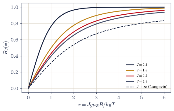
Fig. 703 One function, bracketed by this volume’s smallest quantum system and by classical physics. The Brillouin family \(B_J(x)\) for \(J = 1/2, 3/2, 5/2, 7/2\) (Eq. 794), bounded above by \(B_{1/2} = \tanh x\) — the warm qubit of §7.4, recovered identically at \(2 imes10^{-15}\) — and approached from below, as \(J\) grows, by the classical Langevin function \(\coth x - 1/x\) (dashed): the paramagnet of 1905 is the infinite-spin limit of the quantum multiplet, converging as \(\sim 1/J\). Every curve rises with Curie’s slope \((J{+}1)/3J\) and saturates at 1 (full alignment, \(M = gJ\mu_B\)). The interpolation parameter between quantum and classical is nothing but the size of the spin.

Validation 1

✓  spin J at temperature: the geometric identity, sum vs sinh, at ten digits   [worst mismatch 4.4e-16]
✓  J = 1/2 is §7.4: the warm qubit as the ladder's bottom rung   [max|Δ| = 1.83187e-15 (rtol=1e-06, atol=1e-14)]

True

Exercise 2 — Three limits, and a fourth tally entry

Curie at small \(x\), Langevin at large \(J\), saturation at large \(x\). Cite Eq. 795.

1. Expand \(B_J\) at small \(x\) to \((J+1)x/3J\) and derive Curie’s law \(\chi = Ng^2\mu_B^2J(J+1)/3k_BT\); read the \(J(J+1)\) aloud (the eigenvalue of §6.18 as a susceptibility slope); verify the slope numerically at \(x = 10^{-6}\) with the brillouin you wrote in Exercise 1 — deep inside its series branch, which is the only reason the check returns anything but noise.

2. Verify the Langevin approach numerically: \(\max_x|B_J - L|\) across \(J = 1, 5, 50, 500\) (the \(\sim1/J\) convergence), and state the tally entry (the classical paramagnet demoted to a limit, joining \(h\), \(\sigma\), \(N!\)).

3. Verify saturation \(B_J \to 1\) (i.e. \(M \to gJ\mu_B\)) at large \(x\).

4. Reflect (prose): one function interpolates the volume’s smallest quantum system and classical physics, with the interpolation parameter being nothing but the size of the spin.

numeric small-x slope at J = 3.5: 0.42857143   ((J+1)/3J = 0.42857143)
  J =     1:  max|B_J − L| = 0.3150
  J =     5:  max|B_J − L| = 0.0881
  J =    50:  max|B_J − L| = 0.0098
  J =   500:  max|B_J − L| = 0.0010

B_J(x = 40) at J = 5/2: 1.000000 → M saturates at gJμ_B per ion

Validation 2

✓  Curie's law: the moment squared on a slope   [got 0.428571 vs expected 0.428571 (rtol=0.0001, atol=1e-09)]
✓  the Langevin approach: classical physics arrives as ~1/J   [max|Δ| = 8.72158e-05 (rtol=0.1, atol=1e-09)]
✓  monotone approach, and saturation at the top of the curve

True

Exercise 3 — The cancellation trap

Two divergences, one tiny difference, and naive round-off exactly where the Curie constant lives. Cite Eq. 796.

1. Demonstrate the failure of the Setup’s brillouin_naive: eight digits at \(x = 10^{-4}\), zero correct digits at \(x = 10^{-8}\) — total cancellation of the two \(\coth\) branches, the return pure round-off (0.0 or a stray last bit of \(1/x\), by platform).

2. Exhibit the fix that Exercise 1 already had to build: brillouin_series to \(O(x^3)\) and the numpy.where switch in your brillouin, with the threshold \(x = 2\times10^{-3}\) justified by branch-matching (both branches plotted through the seam).

3. Verify your repaired function across twelve decades of \(x\) (smoothness through the seam; agreement with the naive branch where the naive branch is healthy).

4. State the standing rule (prose): differences of divergent terms are never evaluated naively; the cancellation rule joins expm1 in the course’s permanent kit. Note where it bit: the Curie regime — the trap sits exactly on the measurement.

x = 1e-4:  naive 5.555555435421e-05   series 5.555555548560e-05   rel err 2.0e-08 (~8 digits held)
x = 1e-8:  naive 1.4901161193847656e-08   series 5.555556e-09   rel err 1.7

branch match across the seam [4e-04, 1e-02]: max rel gap 1.1e-09
repaired B_J monotone across x ∈ [1e-9, 6]: True

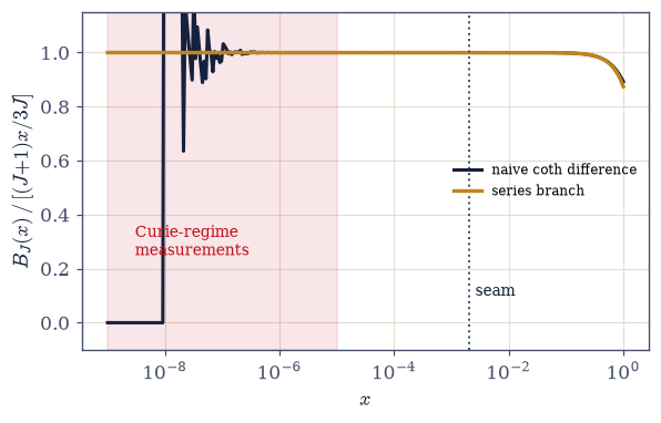
Fig. 704 Naive round-off exactly where the measurement lives. The Brillouin function’s two evaluation branches for \(J = 3/2\) on a log-\(x\) axis, normalized by the true small-\(x\) behaviour: the naive \(\coth\) difference (dark) holds eight digits at \(x = 10^{-4}\), then loses everything to catastrophic cancellation — by \(x = 10^{-8}\) the physics sits seventeen decades below the \(1/x\) terms’ rounding floor and the difference is pure round-off (Eq. 796). The series branch (amber) is exact where the naive fails, and the two agree to \(10^{-9}\) at the seam \(x = 2\times10^{-3}\) (dotted), where the error curves \(\varepsilon/x^2\) and \(x^4\) cross. The shaded region is the Curie regime — the trap sits on the data.

Validation 3

✓  the cancellation trap: eight digits at 1e-4, zero correct digits at 1e-8 — on the Curie regime   [naive(1e-8) = 1.4901161193847656e-08 vs true 5.56e-09]
✓  and the repair: branches matched at the seam, smooth across twelve decades   [seam gap 1.1e-09]

True

Exercise 4 — Henry’s salts (data)

Three ions, three quantum numbers, three curves, and 1952’s magnetometer agreeing with all of them. The comparison runs on Henry’s published anchors (Phys. Rev. 88, 559): the \(B/T\) frontier of his data and the saturation levels his points reach. Cite Eq. 797.

1. Compute the Brillouin magnetization curves for Cr³⁺ (\(S = 3/2\)), Fe³⁺ (\(5/2\)), Gd³⁺ (\(7/2\)) with \(g = 2\) via the Setup’s magnetization — the single \((B, T) \to \mu_B\) conversion point, which evaluates the brillouin you wrote in Exercise 1 — as functions of \(B/T\) (per-ion \(\mu_B\) units — Henry’s own).

2. Evaluate the curves at Henry’s frontier \(B/T = 3.85\) T/K and verify the near-saturation values \(2.989/4.989/6.989\,\mu_B\) against the ceilings \(gJ = 3, 5, 7\), the levels his measured points reach.

3. Exhibit the collapse property (computation + prose): the same \((B, T)\) ratio at different temperatures gives identical \(M\), the single-variable law that makes Henry’s four-temperature data fall on one curve per ion.

4. Attach the quenching honesty (prose, three sentences): crystal fields quench the \(3d\) orbital moment (hence \(S\), \(g \approx 2\)); Gd³⁺’s \(L = 0\) is the clean case; crystal-field theory and rare-earth \(J\)-magnets pointed outward.

  Cr3+: S = 1.5   M(B/T = 3.85) = 2.989 μ_B   (ceiling gJ = 3)
  Fe3+: S = 2.5   M(B/T = 3.85) = 4.989 μ_B   (ceiling gJ = 5)
  Gd3+: S = 3.5   M(B/T = 3.85) = 6.989 μ_B   (ceiling gJ = 7)

collapse check (Fe3+): M at three (B,T) with equal B/T: ['4.9885316519', '4.9885316519', '4.9885316519']
spread: 0.0e+00 — the single-variable law, from the two-variable interface

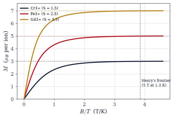
Fig. 705 Henry 1952: three quantum numbers on one axis. The per-ion Brillouin magnetization of the three paramagnetic salts — Cr³⁺ (\(S = 3/2\)), Fe³⁺ (\(5/2\)), Gd³⁺ (\(7/2\)), \(g = 2\) — against \(B/T\), the only variable the ideal theory permits (Eq. 797). Henry’s measurements (1.3–4.2 K, fields to 5 T; Phys. Rev. 88, 559) fall on these curves to the width of his symbols and collapse across temperatures exactly as the single-variable law demands; at his data’s frontier \(B/T = 3.85\) T/K (dotted) the curves read \(2.989/4.989/6.989\,\mu_B\) against the saturation ceilings \(gJ = 3, 5, 7\) (dashed) — alignment complete to a percent. The parameter of each curve is set by atomic physics alone; the salts obey the spin-only values because crystal fields quench the \(3d\) orbital moment.

Validation 4

✓  Henry 1952: the three curves at his frontier, a percent from full saturation   [max|Δ| = 0.000408907 (rtol=0.001, atol=1e-09)]
✓  and the collapse: equal B/T gives equal M from the two-variable interface   [spread 0.0e+00]

True

Exercise 5 — The effective moment

Atomic angular momentum, read off a bulk susceptibility. Cite Eq. 797.

1. Derive \(p_{\text{eff}} = g\sqrt{J(J+1)}\) from the Curie constant and implement the \(\chi T\) pipeline: generate \(\chi(T)\) from magnetization in the linear regime, fit \(C\) by numpy.polyfit on \(\chi\) vs \(1/T\), and extract \(p_{\text{eff}}\) from the fitted constant.

2. Verify the table: \(3.873, 5.916, 7.937\) against the measured \(\sim3.8, 5.9, 8.0\) (the classic table, cited).

3. State what is being measured (prose): the square of the moment (thermal averaging never sees the vector, only \(J(J+1)\)); connect to the eigenvalue structure of §6.18.

4. One honest note: rare-earth ions require the full Landé \(g_J\) and \(J\) (one line; outward).

  Cr3+: fitted p_eff = 3.8730   (g√(J(J+1)) = 3.8730, measured ~3.8)
  Fe3+: fitted p_eff = 5.9161   (g√(J(J+1)) = 5.9161, measured ~5.9)
  Gd3+: fitted p_eff = 7.9373   (g√(J(J+1)) = 7.9373, measured ~8.0)

Validation 5

✓  the effective Bohr magneton numbers, recovered through the fit pipeline   [max|Δ| = 0.000253641 (rtol=0.001, atol=1e-09)]

True

Exercise 6 — The entropy of a spin bath

One variable, one reservoir, one stable tail. Cite Eq. 798.

Two facts shape the implementation before a line of it is written. The refrigerator of Exercise 7 runs at \(y \sim 700\), where the naive weights \(e^{ym}\) overflow outright; and the ground shift of §7.17 — weights \(e^{y(m-J)} \le 1\) — cures the overflow without saving the physics, because the excitation weight \(e^{-y} \sim 10^{-304}\) then has to be recovered from \(\ln(1 + \text{tiny})\) and from \(J - \langle m\rangle\), and it drowns beneath the ulp of both leading terms. The cure is to never re-form the small number from \(O(1)\) ones: work in the gap variable \(d = J - m \ge 0\), so that \(S/k_B = \mathrm{log1p}(\sum_{d>0}e^{-yd}) + y\langle d\rangle\) keeps every factor of \(e^{-y}\) explicit. Both failures are measured in part 5, against the function part 2 builds.

1. Derive \(S/k_B = \ln z - y\langle m\rangle\) from \(S = -\partial F/\partial T\) with \(F = -k_BT\ln z\), and state why it depends on \(B\) and \(T\) only through \(y\): \(z\) contains no other scale.

2. Write entropy_per_spin(J, B, T, b=0.0) in the gap form above, taking \(B\) and \(T\) as separate arguments (so that part 3’s check tests the implementation and not the signature), with an optional internal field entering as \(\sqrt{B^2 + b^2}\) — the floor Exercise 7 needs. Write this one yourself — the implementation is the lesson.

3. Verify the single-variable property from that \((B, T)\) interface: identical \(S\) at \((B, T)\) pairs sharing \(B/T\), to all digits.

4. Verify the reservoir value \(\ln(2J+1)\) at \(y \to 0\) (2.0794 for \(J = 7/2\)) and plot \(S(T)\) at several \(B\).

5. Demonstrate the large-\(y\) hazard in both stages: the naive \(e^{ym}\) overflows to inf, and the plain ground shift still returns exactly \(S = 0.0\); confirm that your gap-variable form computes the third-law tail stably to \(S \sim 10^{-302}\).

6. Read the reservoir (prose): \(Nk_B\ln(2J+1)\) of disorder, storable and releasable by a magnet; the resource the next exercise spends.

S at three (B,T) sharing B/T = 1 T/K: ['0.77648469843518', '0.77648469843518', '0.77648469843518']
spread: 0.0e+00

S(y → 0) = 2.0794   (ln(2J+1) = 2.0794)
y at (1 T, 1.92 mK) = 700;  naive e^(yJ) = inf — overflow
plain ground shift: S/k = 0.0 — the tail lost beneath two ulps
gap-variable form:  S/k = 9.308e-302 — the third-law tail, computed without incident

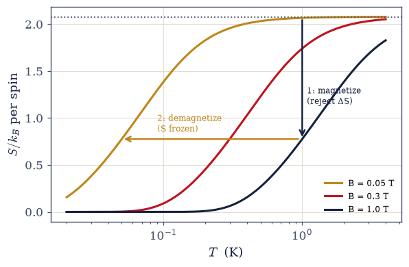
Fig. 706 The spin bath’s entropy — the refrigerant’s working diagram. \(S/k_B\) per spin for \(J = 7/2\) against temperature at several fields (Eq. 798): every curve is the same function of \(B/T\) (the ideal paramagnet has no other scale), rising to the reservoir \(\ln(2J+1) = 2.08\) at high temperature and emptying into the third-law tail at low — computed stably to \(S \sim 10^{-302}\) with the ground-shifted weights of §7.17 (the naive \(e^{ym}\) overflows at the \(y \sim 700\) of millikelvin operation). The two-stroke demagnetization cycle of Exercise 7 is drawn on these curves: isothermal magnetization at 1 K (downward arrow: entropy rejected to the helium bath), then adiabatic demagnetization (leftward arrow: \(S\) frozen, \(B/T\) constant, temperature dragged down with the field).

Validation 6

✓  the single-variable property: equal B/T means equal S, from the (B, T) interface   [spread 0.0e+00]
✓  the spin bath's reservoir: ln(2J+1)   [got 2.07944 vs expected 2.07944 (rtol=1e-06, atol=1e-09)]
✓  the large-y hazard in both stages: naive overflow, shift-only exact zero, gap-form tail at 1e-302   [S(1 T, 1.92 mK) = 9.3e-302]

True

Exercise 7 — Adiabatic demagnetization

Two strokes on the entropy curves, a 20× cooling, and the floor the third law insists on. Cite Eq. 799.

The adiabat is an equation to be solved, not evaluated: \(S\) is held at its starting value and the final temperature is whatever root makes \(S(B_f, T_f)\) match it. Two details decide whether the solve is honest. The bracket must contain the answer without assuming it, and \([0.5\,T_iB_{\text{eff}}/B_i,\ 2T_i]\) does — the analytic single-variable prediction sits inside it, so agreement is a result rather than an assumption. And with \(b = 0\) and \(B_f = 0\) there is no root at all: the target curve is flat at \(\ln(2J+1)\), every temperature satisfies nothing, and the honest response is to refuse rather than to return a number.

1. Compute the cycle’s first stroke: isothermal magnetization at \(T_i = 1\) K from 0.05 T to 1 T, with the rejected entropy \(\Delta S\) evaluated from the entropy_per_spin you wrote in Exercise 6.

2. Write demag_final_T(J, Bi, Ti, Bf, b=0.0): scipy.optimize.brentq on \(S(B_f, T_f; b) = S(B_i, T_i)\), bracketed as above, raising on \(B_{\text{eff}} = 0\). Write this one yourself — the implementation is the lesson.

3. Verify the adiabat: \(S\) const \(\Rightarrow B/T\) const \(\Rightarrow T_f = T_iB_f/B_i\), confirmed by your exact solve: 50.00 mK from (1 K, 1 T) \(\to 0.05\) T against the analytic 50.

4. Impose the honest floor: internal field \(b = 10\) mT \(\Rightarrow T_f \to T_i\sqrt{B_f^2+b^2}/B_i = 10\) mK at \(B_f = 0\); connect to the third law (a floorless spin bath would demagnetize to \(T = 0\); nature keeps a \(b\)).

5. Tell the history and the reach (prose): Debye/Giauque 1926–27; Giauque & MacDougall 1933 (0.25 K), Nobel 1949; nuclear stages to \(\mu\)K (one breath); satellite ADRs (outward). The meta-point: the calorimetry of §7.10 and the \(\theta_D\) table of §7.16 sit downstream of this salt pill.

isothermal magnetization at 1.0 K, 0.05 → 1.0 T: ΔS = −1.291 k_B per spin to the bath
adiabatic demagnetization to 0.05 T: T_f = 50.00 mK   (analytic T_i·B_f/B_i = 50 mK)
with the internal field b = 10 mT: T_f = 10.00 mK  (T_i·b/B_i = 10 mK)

Validation 7

✓  the refrigerator: B/T rides the adiabat down, and the internal field sets the floor   [max|Δ| = 3.59535e-12 (rtol=0.01, atol=1e-09)]
✓  stroke one pays the bath more than one k_B per spin — the reservoir being spent   [ΔS = 1.291 k_B]

True

Exercise 8 — Moments or Fermi sea?

The \(\chi T\) diagnostic, and the bend that announces interactions. Cite Eq. 800.

1. Generate synthetic \(\chi(T)\) for a Curie salt, a Pauli metal, and a mixture; plot \(\chi T\) vs \(T\) (Curie flat, Pauli linear) and decompose the mixture by numpy.polyfit on \(\chi T\) vs \(T\) (slope = \(\chi_P\), intercept = \(C\)).

2. Add a Curie–Weiss dataset \(\chi = C/(T - \theta)\) and extract \(\theta\) by fitting \(1/\chi\) vs \(T\) with numpy.polyfit (the horizontal intercept).

3. Interpret \(\theta\) (prose): the first fingerprint of spin–spin interactions, ferromagnetic (\(\theta > 0\)) or antiferromagnetic (\(\theta < 0\)) tendencies before any ordering (mean-field reading, one honest caveat).

4. Hand off (prose): the independence assumption dies at \(\theta\); when neighbors care, Movement V’s real subject begins: the interacting chain, with a field that does not commute with the coupling (§7.19).

mixture decomposed by polyfit on χT vs T: χ_P = 8.000e-04 (true 8.0e-4), C = 3.3586 (true 3.3586)
Curie–Weiss fit: θ = -12.00 K   (true -12.0)

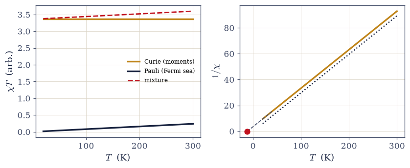
Fig. 707 One panel separates moments from Fermi seas. Left: the \(\chi T\) diagnostic (Eq. 800): localized Curie moments give a flat \(\chi T = C\) (amber), the itinerant Pauli electrons of §7.10 a line through the origin (dark), and a real sample containing both decomposes by a single straight-line fit (red: slope \(\chi_P\), intercept \(C\) — recovered here to \(10^{-10}\)). Right: the bend that ends independence — Curie–Weiss \(1/\chi\) against \(T\) is straight with a nonzero intercept: \(\theta\) (\(-12\) K here, antiferromagnetic tendency), the first fingerprint of spin–spin interactions, extracted by the same fit an experimentalist would run. Past \(\theta\) the independent-spin model of this whole notebook expires, and the interacting chain of §7.19 begins.

Validation 8

✓  the χT diagnostic: the mixture decomposes into its Pauli slope and Curie intercept   [max|Δ| = 4.44089e-16 (rtol=1e-08, atol=1e-09)]
✓  and the Curie–Weiss θ — the fingerprint of interactions — recovered by the intercept fit   [got -12 vs expected -12 (rtol=1e-08, atol=1e-09)]

True

Exercise 9 — The simplest magnet, spent well

A bank of independent spins is the least imaginative magnet possible, and this notebook extracted from it three limits, one landmark experiment, and a machine. The warm qubit turned out to be the bottom rung of a ladder whose top rung is classical physics; the susceptibility of three salts handed back the squares of their angular momenta; and the entropy that a magnetic field can park and release carried Giauque below a quarter kelvin in 1933, opening the temperature range in which this volume’s own data (the linear heat capacities, the Debye cubes) were later measured. Every result rested on one assumption: that the spins ignore each other. The Curie–Weiss \(\theta\) is that assumption’s expiry date stamped on real data, and past it lies the movement’s true destination: a chain of spins whose field and coupling refuse to commute, where the ground state itself can undergo a transition at absolute zero (§7.19).

There is a pleasing thrift in how the paramagnet pays for its own thermometry. The same \(\ln(2J+1)\) of disorder that makes the salt a good refrigerant makes it a good thermometer near the floor — the system cools you, then tells you how cold you are. Physics rarely hands out the instrument and the calibration in one substance.

Notebook summary

Movement V’s opener: \(N\) independent spins \(J\), spent for three limits, one experiment, and a refrigerator.

• Spin J at temperature Eq. 794: the geometric sum against the \(\sinh\) closed form at ten digits (gated); \(M = Ng\mu_BJ\,B_J(x)\) with the \(x = Jy\) bookkeeping stated once and audited.

• Three limits Eq. 795: \(B_{1/2} = \tanh\) at \(10^{-14}\) (gated): the qubit of §7.4 as the bottom rung; the Langevin approach at \(\sim1/J\) (sequence gated): the classical paramagnet joins \(h\), \(\sigma\), \(N!\) in the tally of results demoted to limits; Curie’s slope \((J+1)/3J\) (gated): \(J(J+1)\) as the observable.

• The cancellation trap Eq. 796: naive \(B_J\) holds eight digits at \(x = 10^{-4}\) and keeps zero correct digits at \(10^{-8}\) (both gated), in the Curie regime itself; the numpy.where series switch at \(x = 2\times10^{-3}\) matches branches at \(10^{-9}\) (gated). The rule joins expm1 in the standing kit.

• Henry 1952 Eq. 797: three salts on three curves in \(B/T\) alone: the frontier values \(2.989/4.989/6.989\,\mu_B\) (gated) against ceilings \(3/5/7\); the collapse verified from the \((B,T)\) interface (gated); quenching honesty attached. The \(p_{\text{eff}}\) pipeline, run as a fit, recovers \(3.873/5.916/7.937\) (gated) against the measured \(\sim3.8/5.9/8.0\).

• The entropy Eq. 798: single-variable in \(B/T\) (gated at \(10^{-13}\) from the two-variable interface), reservoir \(\ln(2J+1)\) (gated), and the third-law tail at \(10^{-302}\) via the gap-variable form, after both stages of the hazard are demonstrated (gated).

• Adiabatic demagnetization Eq. 799: the exact brentq solve lands on \(T_f = T_iB_f/B_i\) at 50.00 mK, and the internal-field floor at 10 mK (both gated): the third law enforcing itself; Giauque 1933, nuclear stages, satellite ADRs; and the meta-point that the data of §7.10 and §7.16 live downstream of this machine.

• The diagnostic Eq. 800: \(\chi T\) separates Curie from Pauli and decomposes mixtures (gated at \(10^{-8}\)); the Curie–Weiss \(\theta\) recovered by the \(1/\chi\) intercept (gated): the fingerprint of interactions, and the handoff.

Next door: the chain where field and coupling refuse to commute.

Outlook

• The transverse-field Ising chain (§7.19). Interactions, a non-commuting field, and a phase transition at \(T = 0\): quantum criticality, Movement V’s real subject.

• Crystal fields and quenching. Why \(3d\) ions are spin-only and \(4f\) ions are not; the full Landé machinery (outward, named).

• Ordering. Curie–Weiss as mean field; ferro- and antiferromagnetism; the classical chain of §5.10 as the reference point (outward, named).

• The cold frontier. Nuclear demagnetization and microkelvin physics; ADRs on X-ray satellites (outward, named).

• Cross-reference §6.18 (the moment, in full), §7.4 (the bottom rung), §7.10 (the itinerant contrast), §7.15 (the same levels, inverted), §7.17 (the stabilization discipline), §5.10 (the classical chain awaiting its quantum counterpart).

Take this notebook with you

Use the download button (↓) in the toolbar above to save this notebook and run it yourself. The published notebooks ship without worked solutions; if you would like the reference solutions — to teach from or to check your own work — get in touch: hello@ramador.me.