


3.7 Electromagnetic Induction#
Notebook overview#
Until now the electric field has been conservative. Charges made it, it pointed from them, and the work it did around any closed path was zero, which is exactly what let us define a single-valued scalar potential \(V\) in §3.2. This notebook is where that picture breaks, and it breaks on purpose: a changing magnetic field makes an electric field, and that induced field does not emanate from charges, it circulates. Its line integral around a loop is no longer zero. That one fact, Faraday’s law of induction, is the conceptual hinge of the volume.
We build it in stages. First the integral law: a changing magnetic flux through a loop drives an electromotive force, \(\mathcal{E}=-d\Phi_B/dt\), with the minus sign of Lenz’s law enforcing energy conservation. Then the same physics seen from a moving conductor (motional EMF), and the payoff every power grid runs on, the AC generator. Then the local form, \(\nabla\times\mathbf E=-\partial_t\mathbf B\), obtained from the integral law by Stokes’ theorem. This is the third of Maxwell’s four equations and the first to couple \(\mathbf E\) and \(\mathbf B\) dynamically: where §3.2 had \(\nabla\times\mathbf E=0\), we now find \(\nabla\times\mathbf E\neq0\), so \(\mathbf E\) is no longer the gradient of a potential alone. We make that failure of path-independence concrete and numerical, the very property §3.2 warned would not survive induction.
Finally the practical consequences: inductance (a circuit’s flux opposing changes in its own current, and the mutual coupling between circuits), the magnetic field energy \(\tfrac12 LI^2\) that mirrors the electric field energy of §3.2, and the eddy-current braking that makes a magnet drift slowly down a copper pipe. We close by collecting three of the four field equations, with the fourth, and light itself, one notebook away.
Everything is in SI units, with \(\mu_0=4\pi\times10^{-7}\,\)T·m/A. Induction is the place motion returns as genuine physics, so exactly one figure here is animated, the changing flux of Exercise 1; everything else is a still.
How to read the checks. Each exercise ends with a
validatecall against an independent fact: an induced EMF matching \(-d\Phi/dt\), a Lenz sign opposing the change, a numerical curl equal to \(-\partial_t\mathbf B\), a circulation that refuses to vanish, a mutual inductance matching the coaxial-loop formula. A ✓ is strong evidence; a ✗ is a prompt to locate the discrepancy, not a verdict.A numerical-differentiation note. Several checks differentiate a sampled signal with
numpy.gradient. Its one-sided stencils at the first and last sample are less accurate than the centred stencil used in the interior, so we validate on the interior (excluding the two end points), the same array-edge subtlety met when taking divergences and curls on a finite grid.
Theory in brief#
Faraday’s law#
The magnetic flux through a loop spanning a surface \(S\) is \(\Phi_B=\int_S \mathbf B\cdot d\mathbf A\). Faraday’s law says a changing flux drives an electromotive force around the loop’s boundary,
The flux can change three ways: \(\mathbf B\) itself changes in time, the loop’s area changes, or the loop moves or rotates in a non-uniform or angled field. All three appear below.
Lenz’s law: the minus sign#
The sign in Eq. 225 is Lenz’s law:
If the flux is increasing, the induced current makes a field opposing the increase; if decreasing, it props the flux up. This is energy conservation in disguise: a current that reinforced the change would amplify itself without limit and deliver free energy. The induced EMF therefore always carries the sign opposite to \(d\Phi_B/dt\).
Motional EMF#
When a conductor moves through a field, the magnetic force \(q\,\mathbf v\times\mathbf B\) on its charge carriers pushes them along the conductor, acting as a battery:
For a bar of length \(L\) sliding at speed \(v\) perpendicular to a uniform field \(B\) this is \(\mathcal{E}=BLv\), and it agrees exactly with the flux rule Eq. 225 applied to the growing circuit area, two pictures of one phenomenon.
The differential form: the hinge#
Stokes’ theorem turns \(\oint\mathbf E\cdot d\boldsymbol\ell=-d\Phi_B/dt\) into a local statement,
This is the hinge of the volume. In electrostatics \(\nabla\times\mathbf E=0\): the field is conservative, a scalar potential exists, and \(\oint\mathbf E\cdot d\boldsymbol\ell=0\), the path-independence of §3.2. The moment \(\mathbf B\) varies in time, \(\nabla\times\mathbf E\neq0\): the line integral around a loop is no longer zero, \(\mathbf E\) is no longer conservative, and a single-valued scalar potential no longer suffices. The induced field circulates in closed loops; it does not start or end on charges. This is the third of Maxwell’s four equations, and the first that couples \(\mathbf E\) and \(\mathbf B\) dynamically.
Inductance and magnetic energy#
A circuit’s own current makes a flux through itself; the proportionality is the self-inductance \(L\), and \(\mathcal{E}=-L\,dI/dt\). Between two circuits the mutual inductance \(M\) relates the current in one to the flux it sends through the other,
Establishing a current against the induced back-EMF stores energy \(\tfrac12 LI^2\) in the field, with density \(u=B^2/2\mu_0\), the magnetic mirror of the electric field energy \((\varepsilon_0/2)|\mathbf E|^2\) of §3.2.
Toward the unified potential (3.8)#
Once \(\nabla\times\mathbf E\neq0\), the field cannot come from \(V\) alone. The fix uses the vector potential of §3.6 alongside the scalar one, \(\mathbf E=-\nabla V-\partial_t\mathbf A\), so that \(V\) and \(\mathbf A\) together carry the field. That is the full gauge structure assembled in §3.8; here we only plant the pointer.
Setup#
Data and instruments only: the vacuum permeability and the series palette, the flux of a uniform field through a flat loop (the formula \(\Phi=BA\cos\theta\) the problems hand you, transcribed), the ring geometry the mutual-inductance problem specifies, and two pieces of machinery you already built by hand in §3.6 — the Biot–Savart integrator of its Exercise 1 and the numerical curl of its Exercise 6, the latter restated here as the one surviving component on a plane. No new method hides here: every EMF below is obtained by differentiating, in the exercise that needs it, a flux you assemble there. No randomness appears anywhere in this notebook.
The Setup below holds this notebook’s data and instruments — nothing you are asked to build. It is collapsed so the building stays yours; expand it whenever you want the details.
Exercise 1 — Faraday’s law: a changing flux (worked)#
The simplest induction experiment holds a loop still and changes the field through it. Take a fixed planar loop of area \(A=0.01\,\mathrm{m}^2\) in a spatially uniform but time-varying field \(B(t)=B_0\sin(\omega t)\) with \(B_0=0.5\,\)T and \(\omega=2\pi\cdot 50\,\mathrm{s}^{-1}\), the field through the loop (Fig. 247). The flux is \(\Phi_B(t)=A\,B(t)\), and Faraday’s law Eq. 225 predicts an EMF \(\mathcal{E}=-d\Phi_B/dt=-A B_0\omega\cos(\omega t)\). Motion is the content here, so this is the one place in the notebook that earns an animation: watching the field through the loop oscillate while the flux and the induced EMF build their curves, a quarter-period apart, is the whole of Faraday’s law in one picture.
Sample \(\Phi_B(t)\) on a uniform time grid over two periods, differentiate it numerically with
numpy.gradientto get \(\mathcal{E}=-d\Phi_B/dt\), and compare to the closed form \(-AB_0\omega\cos(\omega t)\).Validate on the interior of the time array (excluding the two end samples, where
numpy.gradientfalls back to one-sided differences).Animate the oscillating field beside the flux and EMF curves as they are traced out (Fig. 248).
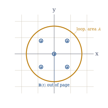
Fig. 247 A fixed planar loop of area \(A\) (amber) threaded by a spatially uniform, time-varying field \(\mathbf B(t)=B_0\sin(\omega t)\,\hat{\mathbf z}\) pointing out of the page (blue \(\odot\)). As \(B(t)\) rises and falls, the flux \(\Phi_B=B(t)A\) changes and, by Faraday’s law, drives an EMF \(\mathcal{E}=-d\Phi_B/dt\) around the loop. Nothing moves; only the field strength changes.#
peak EMF |ℰ| = 1.5708 V (= A B₀ω)
max |ℰ_numeric − ℰ_closed| on the interior = 1.03e-05 V
Validation 1#
✓ the induced EMF equals −dΦ/dt (interior, away from the gradient's edge stencils) [max|Δ| = 1.03457e-05 (rtol=0.001, atol=1e-09)]
True
Fig. 248 Animation of Faraday’s law: the left panel shows the field \(B(t)=B_0\sin(\omega t)\) through a fixed loop (arrow length and colour \(\propto B\), blue out of the page, red into it); the right panel traces the flux \(\Phi_B(t)\) and the induced EMF \(\mathcal{E}(t)=-d\Phi_B/dt\) as they build. The EMF peaks exactly when the flux crosses zero (fastest change) and vanishes at the flux extrema, the quarter-period lag that is Faraday’s law made visible.#
Exercise 2 — Lenz’s law and the sign (worked)#
The minus sign in Eq. 225 is not bookkeeping; it is Lenz’s law Eq. 226, and it encodes energy conservation. The induced EMF, and the current it drives, always opposes the change in flux: when \(\Phi_B\) is increasing the induced current fights the increase, when decreasing it props the flux up. A current that did the opposite would reinforce its own cause and manufacture energy from nothing. At the flux extrema \(d\Phi_B/dt\) passes through zero and its sign carries no information, so those instants have to be masked out; the threshold used below is 1% of the peak rate.
Form \(d\Phi_B/dt\) with
numpy.gradientfrom the flux \(\Phi_B(t)\) you sampled in Exercise 1.Confirm that the induced EMF \(\mathcal{E}=-d\Phi_B/dt\) carries the opposite sign to \(d\Phi_B/dt\) wherever the change is non-negligible, that is, \(\operatorname{sign}\mathcal{E}=-\operatorname{sign}(d\Phi_B/dt)\).
samples with appreciable dΦ/dt: 1988 of 2000
induced EMF opposes the change everywhere there: True
Validation 2#
✓ the induced EMF opposes the change in flux (Lenz's law: sign ℰ = −sign dΦ/dt)
True
Exercise 3 — ∇×E = −∂B/∂t: the field stops being conservative (worked)#
Here is the hinge. Confine a uniformly increasing field to a cylinder of radius
\(a=0.1\,\)m along \(\hat{\mathbf z}\), with \(dB/dt=1.0\,\mathrm{T/s}\). Symmetry forces the
induced electric field to be azimuthal, circling the axis with
\(E_\varphi(r)=-\tfrac{r}{2}\,dB/dt\), so in Cartesian components
\(\mathbf E=\tfrac12\frac{dB}{dt}\,(y,\,-x,\,0)\) (Fig. 249). This
field winds in closed loops and points at no charge. What comes out of the
measurement is precisely the property §3.2 said would fail
once induction entered: the work around a closed loop is no longer zero, \(\mathbf E\)
is no longer conservative, and no single-valued scalar potential can describe it
(Fig. 250). The operator doing the measuring is the numerical
curl you built in §3.6 (its Exercise 6), restated in Setup
as curl_z for the one component a planar field leaves standing.
Build \(\mathbf E\) on a 3-D grid and take its curl numerically with
curl_z; confirm the \(z\)-component equals \(-dB/dt\) everywhere, nonzero.Integrate \(\oint\mathbf E\cdot d\boldsymbol\ell\) around a circle of radius \(r_0=0.05\,\)m with
numpy.trapezoidand confirm it equals \(-d\Phi_B/dt=-\pi r_0^2\,dB/dt\neq0\).
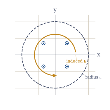
Fig. 249 A cylinder of radius \(a\) (dashed) carrying a uniformly increasing field \(\mathbf B(t)\) out of the page (\(dB/dt>0\), blue \(\odot\)). The induced electric field (amber) is azimuthal, \(E_\varphi=-\tfrac{r}{2}\,dB/dt\), circulating in closed loops around the axis rather than pointing toward any charge. The circulation \(\oint\mathbf E\cdot d\boldsymbol\ell\) around the loop of radius \(r_0\) equals \(-d\Phi_B/dt\neq0\).#
(∇×E)_z (interior mean) = -1.0000 vs −dB/dt = -1.0000
∮E·dℓ = -7.853982e-03 V vs −dΦ/dt = -7.853982e-03 V
Validation 3#
✓ ∇×E = −∂B/∂t (nonzero — the induced E is not conservative) [got -1 vs expected -1 (rtol=0.0001, atol=1e-09)]
✓ ∮E·dℓ = −dΦ/dt ≠ 0, breaking the electrostatic path-independence of §3.2 [got -0.00785398 vs expected -0.00785398 (rtol=0.001, atol=1e-09)]
True
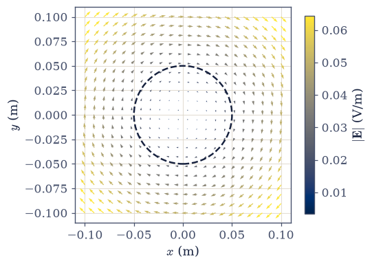
Fig. 250 The induced electric field \(\mathbf E=\tfrac12(dB/dt)(y,-x)\) in the \(z=0\) plane (ecp.draw.field_quiver, arrow length and colour \(\propto|\mathbf E|\)). The field circulates in closed loops about the axis: it begins and ends nowhere, the visual signature of \(\nabla\times\mathbf E\neq0\). Unlike the radial Coulomb field of §3.1, this field is sourced by a changing \(\mathbf B\), not by charge.#
Exercise 4 — The AC generator: a rotating loop (worked)#
Spin a loop in a steady field and the flux changes because the loop’s orientation does: this is how almost all of the world’s electricity is made. Take \(N=100\) turns of area \(A=0.01\,\mathrm{m}^2\) rotating at \(\omega=2\pi\cdot50\,\mathrm{s}^{-1}\) in a uniform field \(B=0.2\,\)T (Fig. 251). The flux per turn is \(B A\cos(\omega t)\), so \(\Phi_B=NBA\cos(\omega t)\) and Faraday’s law gives \(\mathcal{E}=-d\Phi_B/dt=NBA\omega\sin(\omega t)\), a sinusoidal AC output with peak \(NBA\omega\). The flux and the EMF come out a quarter-period (90°) apart, the defining signature of a generator (Fig. 252), and this sinusoidal EMF is exactly the source that will drive the AC RLC circuits of §3.11.
Compute \(\Phi_B(t)=NBA\cos(\omega t)\) over two periods and differentiate it with
numpy.gradientto get \(\mathcal{E}\).Confirm it against the closed form \(NBA\omega\sin(\omega t)\) on the interior of the time array, reusing the
interiorslice of Exercise 1.
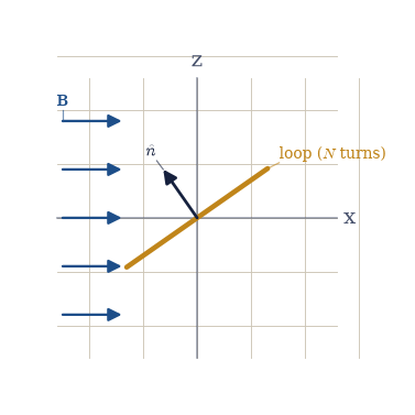
Fig. 251 The AC generator: a loop of \(N\) turns and area \(A\), normal \(\hat{\mathbf n}\) at angle \(\theta=\omega t\) to a uniform field \(\mathbf B\) (blue), rotating at angular speed \(\omega\). The flux per turn is \(BA\cos\omega t\), so spinning the loop modulates the flux and, by Faraday’s law, drives the sinusoidal EMF \(\mathcal{E}=NBA\omega\sin\omega t\). Shown edge-on in the \(x\)–\(z\) plane.#
peak EMF = 62.8319 V (= NBAω)
max |ℰ_numeric − NBAω sin ωt| on the interior = 4.14e-04 V
Validation 4#
✓ the rotating loop generates sinusoidal AC, ℰ = NBAω sin(ωt) (interior) [max|Δ| = 0.00041383 (rtol=0.01, atol=1e-09)]
True
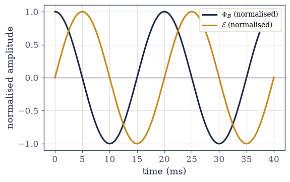
Fig. 252 Generator output over two periods: the flux \(\Phi_B=NBA\cos\omega t\) (dark) and the induced EMF \(\mathcal{E}=NBA\omega\sin\omega t\) (amber), each normalised to its peak. They are a quarter-period (90°) out of phase: the EMF is largest when the flux sweeps through zero (the orientation changing fastest) and zero when the flux is extremal. This phase relationship is the hallmark of AC generation.#
Exercise 5 — Motional EMF: the sliding bar (student)#
Flux can change with no change in the field at all, simply because the circuit’s area grows. A conducting bar of length \(L=0.2\,\)m slides at speed \(v=5\,\)m/s along parallel rails in a uniform field \(B=0.5\,\)T perpendicular to the plane of the circuit (Fig. 253). Two pictures give the same EMF. The flux rule Eq. 225: the enclosed area grows at \(L v\), so \(|d\Phi_B/dt|=BLv\). The force picture Eq. 227: each carrier feels \(q\,\mathbf v\times\mathbf B\), an effective field of magnitude \(vB\) along the bar, which integrated over its length \(L\) gives an EMF \(vBL\).
Compute the motional EMF from the flux rule (the rate of area change times \(B\)).
Compute it again from the \(\mathbf v\times\mathbf B\) force integrated along the bar (
numpy.trapezoid).Confirm they agree and both equal \(BLv\).
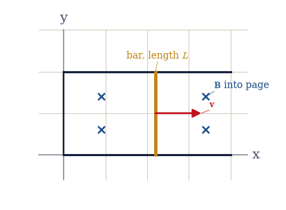
Fig. 253 Motional EMF: a conducting bar of length \(L\) (amber) slides at velocity \(\mathbf v\) along two rails in a uniform field \(\mathbf B\) into the page (blue \(\otimes\)). The circuit area grows at rate \(Lv\), so the flux changes at \(BLv\); equivalently the force \(q\,\mathbf v\times\mathbf B\) drives the carriers along the bar. Both give \(\mathcal{E}=BLv\).#
flux rule: ℰ = B·(L v) = 0.5000 V
force ∫(v×B)·dℓ = 0.5000 V BLv = 0.5000 V
Validation 5#
✓ the motional EMF is BLv [got 0.5 vs expected 0.5 (rtol=1e-06, atol=1e-09)]
✓ the v×B force picture and the flux rule give the same motional EMF [got 0.5 vs expected 0.5 (rtol=1e-06, atol=1e-09)]
True
Exercise 6 — Mutual inductance of coaxial loops (worked)#
When two circuits share flux, the current in one induces an EMF in the other, with the coupling set by the mutual inductance \(M\) Eq. 229. Take two coaxial loops, a large one of radius \(r_1=0.1\,\)m and a small one of radius \(r_2=0.01\,\)m on the same axis, separated by \(z=0.05\,\)m (Fig. 254). For a small inner loop the field is nearly uniform across it, so the dipole/on-axis formula gives \(M=\mu_0\pi r_1^2 r_2^2/\bigl(2(r_1^2+z^2)^{3/2}\bigr)\). That closed form is the check; the measurement runs on the Biot–Savart integrator you wrote in §3.6 (its Exercise 1), restated in Setup.
Drive unit current around loop 1 and evaluate the field it makes at loop 2’s centre with
biot_savart.Multiply \(B_z\) by loop 2’s area \(\pi r_2^2\) — the small-loop approximation — to get the flux through loop 2 per unit current, which is \(M\), and compare it to the closed form above.
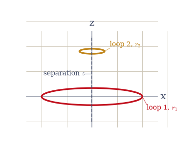
Fig. 254 Two coaxial loops on the \(z\)-axis: a large loop of radius \(r_1\) in the plane \(z=0\) (red) and a small loop of radius \(r_2\) at height \(z\) (amber), shown in the \(x\)–\(z\) plane. A current in loop 1 sends a magnetic flux through loop 2; the flux per unit current is the mutual inductance \(M\). The dashed axis is the common symmetry axis.#
B_z at loop 2 (per amp) = 4.495947e-06 T/A
M (from Biot–Savart flux) = 1.412444e-09 H
M (coaxial-loop formula) = 1.412423e-09 H
Validation 6#
✓ the mutual inductance matches the coaxial-loop formula [got 1.41244e-09 vs expected 1.41242e-09 (rtol=0.01, atol=1e-09)]
True
Exercise 7 — Eddy currents and a magnet falling through a copper pipe (student)#
Lenz’s law has a famous, almost magical demonstration: drop a magnet down a copper pipe and it floats down in slow motion. As the magnet falls, the flux through each ring of the pipe changes, inducing circulating eddy currents that, by Lenz’s law, oppose the change, which means they pull back on the magnet (Fig. 255). The retarding force grows with speed, so the magnet reaches a terminal velocity at which gravity and the magnetic drag balance. The model here is the simplest one that shows the effect: the speed \(v\) (downward, positive) obeys \(m\,\dot v = mg - k\,v\), a linear drag standing in for the induced EMF, with mass \(m=0.01\,\)kg, drag coefficient \(k=0.5\,\)kg/s and \(g=9.81\,\mathrm{m/s^2}\). Setting \(\dot v=0\) gives the terminal speed \(v_\infty=mg/k\) that the integration has to reproduce.
Write the right-hand side \(\dot v = g - (k/m)\,v\) as a
solve_ivpcallable (the time argument goes unused, but the solver requires it).Integrate from rest with
scipy.integrate.solve_ivp(theDOP853high-order Runge–Kutta) and confirm the speed approaches \(v_\infty=mg/k\) (Fig. 256).
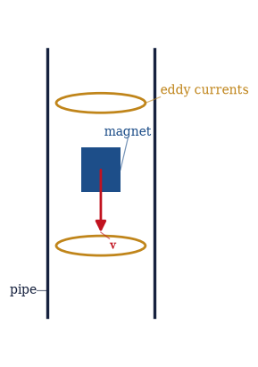
Fig. 255 A magnet falling through a conducting pipe. Its motion changes the flux through each ring of the pipe, inducing circulating eddy currents (amber) that, by Lenz’s law, oppose the change and so exert a retarding force on the magnet (red, opposing \(\mathbf v\)). The drag grows with speed until it balances gravity at the terminal velocity.#
terminal velocity v∞ = mg/k = 0.1962 m/s
final integrated speed = 0.1962 m/s
Validation 7#
✓ eddy-current damping gives a terminal velocity (the magnet falls slowly) [got 0.1962 vs expected 0.1962 (rtol=0.01, atol=1e-09)]
True
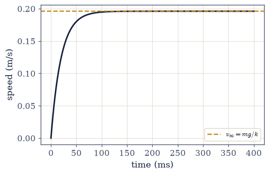
Fig. 256 The falling magnet’s speed against time, from scipy.integrate.solve_ivp (DOP853). Starting from rest it accelerates, but the eddy-current drag grows with speed until it cancels gravity, and the speed levels off at the terminal value \(v_\infty=mg/k\) (dashed). This exponential approach to a slow terminal speed is why a magnet drifts, rather than drops, through a copper pipe.#
Exercise 8 — Energy stored in the magnetic field (student)#
Building a current against the induced back-EMF takes work, and that work is stored in the magnetic field as energy \(\tfrac12 LI^2\), the magnetic mirror of the electric field energy of §3.2. For a long solenoid of \(n\) turns per metre, radius \(R\), length \(\ell\) carrying current \(I\), the interior field is \(B=\mu_0 nI\) (Ampère, §3.6) and the self-inductance is \(L=\mu_0 n^2(\pi R^2)\ell\) (Fig. 257). The two routes to the energy — the circuit’s \(\tfrac12 LI^2\) and the volume integral of the field’s own density — must agree, the field-energy bookkeeping of §3.2 carried over to magnetism. The numbers here are \(n=1000\,\mathrm{m^{-1}}\), \(R=0.02\,\)m, \(\ell=0.4\,\)m and \(I=2\,\)A.
Compute the circuit energy \(\tfrac12 LI^2\).
Independently, integrate the field-energy density \(u=B^2/2\mu_0\) over the solenoid’s interior volume with
numpy.trapezoid, and confirm the two agree.
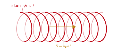
Fig. 257 A solenoid (ecp.draw.solenoid) of \(n\) turns per metre, radius \(R\) and length \(\ell\) carrying current \(I\). Its interior field \(B=\mu_0 nI\) stores energy at density \(u=B^2/2\mu_0\); integrated over the interior volume this equals the circuit energy \(\tfrac12 LI^2\) with \(L=\mu_0 n^2(\pi R^2)\ell\).#
L = 6.316547e-04 H, B = 2.513274e-03 T
½LI² = 1.263309e-03 J
∫ B²/2μ₀ dV (interior) = 1.263309e-03 J
Validation 8#
✓ the field energy ∫(B²/2μ₀) dV equals the circuit energy ½LI² [got 0.00126331 vs expected 0.00126331 (rtol=0.001, atol=1e-09)]
True
Exercise 9 — Three of four, and the coupling begins#
Step back and collect the field equations. After electrostatics, magnetostatics and now induction, three of the four are in hand, and one of them has just changed character:
The third equation is new in kind: for the first time a time derivative couples the two fields, a changing \(\mathbf B\) making an \(\mathbf E\). The fourth is still the static Ampère law, and it is incomplete: consistency with charge conservation will force a symmetric term, a changing \(\mathbf E\) making a \(\mathbf B\), the displacement current of §3.8. Add that one term and the equations close into a self-sustaining system whose solutions propagate: light.
One structural consequence is already unavoidable. With \(\nabla\times\mathbf E\neq0\) the field can no longer come from a scalar potential alone; it needs the scalar and vector potentials together, \(\mathbf E=-\nabla V-\partial_t\mathbf A\), the full gauge picture set up in §3.8. Nothing in this notebook varies \(\mathbf E\) in time, so the displacement-current twin \(\partial_t\mathbf E\) is still identically zero here; we are one term, and one notebook, from light.
Tabulate the three field equations now in hand alongside the incomplete fourth.
Confirm quantitatively, from the interior curl you measured in Exercise 3, that the induced field satisfies \(\nabla\times\mathbf E = -\partial_t\mathbf B\) — the one dynamic term now switched on.
∇·E = ρ/ε₀ — Gauss (§3.3)
∇·B = 0 — no monopoles (§3.6)
∇×E = −∂B/∂t — Faraday (here — NEW coupling)
∇×B = μ₀J (+ ∂E/∂t?) — Ampère (§3.6) — completed in §3.8
measured: (∇×E)_z = -1.0000 vs −dB/dt = -1.0000 (residual 0.00e+00); the ∂E/∂t twin awaits §3.8
Validation 9#
✓ the one dynamic term switched on, measured: ∇×E = −∂B/∂t; its ∂E/∂t twin awaits §3.8 [got 0 vs expected 0 (rtol=1e-06, atol=0.0001)]
True
Notebook summary#
Faraday’s law Eq. 225: a changing flux drives \(\mathcal{E}=-d\Phi_B/dt\); we differentiated a sampled flux with
numpy.gradientand matched the closed form on the interior (Exercise 1, the warranted animation).Lenz’s law Eq. 226: the induced EMF opposes the change in flux, energy conservation made into a sign (Exercise 2).
The hinge Eq. 228: for a region of changing \(\mathbf B\) the induced \(\mathbf E\) circulates, \(\nabla\times\mathbf E=-\partial_t\mathbf B\neq0\) and \(\oint\mathbf E\cdot d\boldsymbol\ell\neq0\), breaking the path-independence of §3.2 (Exercise 3).
The AC generator (Exercise 4): a rotating loop gives \(\mathcal{E}=NBA\omega \sin\omega t\), sinusoidal AC from first principles, the source for §3.11.
Motional EMF Eq. 227: the sliding bar gives \(BLv\) by the flux rule and the \(\mathbf v\times\mathbf B\) force alike (Exercise 5).
Inductance and energy Eq. 229: the mutual inductance of coaxial loops from a Biot–Savart flux (Exercise 6), and the magnetic field energy \(\tfrac12 LI^2 = \int B^2/2\mu_0\,dV\) (Exercise 8); eddy-current braking and a terminal velocity for a magnet in a pipe (Exercise 7).
Three of four field equations assembled, with \(\nabla\times\mathbf E\) now dynamic and the displacement current of §3.8 the last piece before light (Exercise 9).
Outlook#
The betatron. Induction is not just a generator trick: the circulating induced \(\mathbf E\) of Exercise 3 can accelerate particles. A betatron ramps a magnetic field to drive electrons around a ring with no electrodes at all, the induced field doing the work.
The transformer. Mutual inductance (Exercise 6) at industrial scale: two coils sharing a flux step voltages up or down, the device that makes the AC power grid practical.
AC circuits and impedance (§3.11). The sinusoidal EMF of the generator (Exercise 4) is exactly the source that drives the RLC resonator; inductors there contribute a reactance \(\omega L\), the circuit face of the \(\tfrac12 LI^2\) energy met here.
The potential formulation and the Lorenz gauge (§3.8). Once \(\nabla\times\mathbf E\neq0\) we need \(\mathbf E=-\nabla V-\partial_t\mathbf A\); the gauge arc begun in §3.6 continues there and closes with electromagnetic waves.
Superconductors and flux quantization (Vol VI). A persistent current flows forever with no driving EMF, and the trapped flux comes in discrete quanta \(h/2e\), a macroscopic quantum effect that this classical picture can only point toward.