6.3 Dirac Notation, Bases, and Spectral Decomposition

Elementary Computational Physics

Volume VI — Quantum Mechanics Notebook 6.3

The language. We give the inner product and the operators of the last two notebooks their proper notation — kets, bras, and the outer product — and find it is not shorthand but a calculus. Projectors extract components, the resolution of the identity lets us expand in any basis at will, and the spectral decomposition turns any function of an operator into a function of its eigenvalues. With this in hand, the physics can begin.

Level · advanced   •   Est. · 150–190 min

Raymond Amador v1.4.0  ·  2026-07-31  ·  CC BY 4.0 (text) / MIT (code)

Notebook overview

Two notebooks ago we built the space; one notebook ago we built the operators. This notebook builds the language in which the rest of the volume is written — Dirac’s notation of kets and bras — and the surprise it holds is that the notation is not a convenience laid on top of the mathematics but a calculus: a small set of symbols whose manipulation rules do the work for us. It is the closing notebook of Movement 0, the mathematical arsenal, and by its end the formalism is complete and the physics can begin.

The notebook also keeps two promises. In §6.1 we used \(\langle u|v\rangle\) as shorthand and promised that the bra \(\langle u|\) would later become an object in its own right; here it does — a dual vector, the linear functional “take the inner product with \(u\).” In §6.2 we wrote the spectral theorem as a matrix factorization \(A=V\Lambda V^{\dagger}\) and promised an outer-product form; here it arrives as \(A=\sum_\lambda\lambda\,|\lambda\rangle\langle\lambda|\), a Hermitian operator written as its eigenvalues times the projectors onto its eigenvectors. After this notebook there are no remaining notation deferrals in the arsenal.

Three constructions carry the whole calculus, and the notebook is built around them. The projector \(|e\rangle\langle e|\) extracts the component of a state along \(|e\rangle\). The resolution of the identity \(\sum_i|e_i\rangle\langle e_i|=I\) is the compact statement that any state expands in any orthonormal basis — and the single most useful move in the formalism is to insert the identity anywhere a change of basis is wanted. The spectral decomposition \(A=\sum_i\lambda_i|\lambda_i \rangle\langle\lambda_i|\) is “diagonalize” in its cleanest dress, and it makes any function of an operator trivial: apply the function to the eigenvalues. That last fact is the general machinery behind the exponential map of §6.2 and behind the time-evolution operator \(U(t)=e^{-iHt/\hbar}\) that will run all of dynamics (§6.7).

As in every Volume VI notebook, each exercise opens with a crystal-clear statement and enumerated parts that name the exact operation to run — numpy.outer (with numpy.conj for the bra) to build \(|u\rangle\langle v|\), explicit projector and resolution-of-identity construction, numpy.linalg.eigh for the spectral data, scipy.linalg.expm to cross-check the spectral exponential — so the method is never something to reverse-engineer.

A word on what closes here. This notebook resolves the two boundaries the arsenal carried. The bra \(\langle u|\) is now a dual vector (as promised in §6.1), and the outer product, projectors, the projector form of the spectral theorem, and functions of operators are all developed (as promised in §6.2). What we deliberately do not do is the physics: the projector is the mathematics of a measurement, but the measurement postulate itself — outcomes, probabilities, collapse — is §6.5. We build the apparatus here and let the physics out in the next movement.

How to read the checks. Each exercise closes with a validate call against an independent fact: the outer product acting as an operator; a projector’s idempotence, Hermiticity, and rank; the resolution of the identity to machine precision; a change of basis preserving eigenvalues and inner products; the spectral decomposition reconstructing a Hermitian operator from its eigen-projectors; a function of an operator matching scipy.linalg.expm and a square root squaring back; and a qubit’s outcome-weights summing to one in two different bases. A ✓ is strong evidence; a ✗ is a prompt to locate the discrepancy.

Scope. Finite-dimensional, orthonormal bases throughout. The measurement postulate is §6.5; the Stern–Gerlach experiment and the two-state system that open the physics are §6.4; the time-evolution operator is §6.7; the Bloch sphere is §6.8. See Sakurai & Napolitano (Ch. 1); Dirac, The Principles of Quantum Mechanics; and Notebooks §6.1 (the inner product), §6.2 (the spectral theorem, the exponential map).

Theory in brief

Kets, bras, and the dual space

A ket \(|\psi\rangle\) is a state vector, a column of complex numbers. A bra \(\langle\phi|\) is the linear functional that eats a ket and returns the number \(\langle\phi|\psi\rangle\) — “take the inner product with \(\phi\).” The bras form the dual space; in components a bra is the conjugate-transpose row vector, the adjoint of the ket,

(501)\[\begin{split}|\psi\rangle=\begin{pmatrix}\psi_1\\\vdots\\\psi_n\end{pmatrix},\qquad \langle\phi|=(\phi_1^{*},\dots,\phi_n^{*}),\qquad \langle\phi|\psi\rangle=\sum_i\phi_i^{*}\psi_i .\end{split}\]

This is the meaning deferred from §6.1: the inner product is a bra acting on a ket.

The outer product

Multiplied the other way, \(|u\rangle\langle v|\) is an operator. Acting on a ket it gives

(502)\[\big(|u\rangle\langle v|\big)\,|w\rangle=\langle v|w\rangle\,|u\rangle ,\]

“measure the overlap with \(v\), output that much of \(u\).” In components it is numpy.outer(u, numpy.conj(v)). The inner product \(\langle v|u\rangle\) is a number; the outer product \(|u\rangle \langle v|\) is an operator. This is the construction deferred from §6.2.

Projectors

For a normalized \(|e\rangle\), the operator

(503)\[P=|e\rangle\langle e|,\qquad P|\psi\rangle=\langle e|\psi\rangle\,|e\rangle,\qquad P^2=P,\quad P=P^{\dagger},\quad \text{eigenvalues }\{0,1\} ,\]

is the projector onto the \(e\)-direction: it keeps only the part of \(|\psi\rangle\) along \(|e \rangle\). Projectors are idempotent (\(P^2=P\) — projecting twice is projecting once), Hermitian, and rank-1. Physically the projector is the mathematical content of a measurement (the postulate is §6.5).

The resolution of the identity

For any orthonormal basis \(\{|e_i\rangle\}\),

(504)\[\sum_i|e_i\rangle\langle e_i|=I,\qquad |\psi\rangle=\sum_i|e_i\rangle\langle e_i|\psi\rangle=\sum_i c_i|e_i\rangle,\quad c_i=\langle e_i|\psi\rangle .\]

This compact identity is “every state expands in the basis” — recovering the expansion coefficients of §6.1, now as projections. The trick that makes the notation flow is to insert the identity anywhere a basis change or expansion is wanted.

Change of basis as a unitary

Changing from one orthonormal basis to another is a unitary \(U\) whose columns are the new basis vectors; components and operators transform as

(505)\[\psi'=U^{\dagger}\psi,\qquad A'=U^{\dagger}AU,\qquad \text{eigenvalues and inner products preserved} .\]

A change of basis is a passive relabelling, not a physical change (cf. the unitary operators of §6.2).

The spectral decomposition in projector form

The spectral theorem of §6.2, \(A=V\Lambda V^{\dagger}\), is exactly

(506)\[A=\sum_i\lambda_i\,|\lambda_i\rangle\langle\lambda_i|,\qquad P_iP_j=\delta_{ij}P_i,\quad \sum_iP_i=I ,\]

a Hermitian operator as its eigenvalues times the projectors onto its eigenvectors. The spectral projectors are orthogonal and resolve the identity. This is the cleanest statement of “diagonalize,” and the form the measurement postulate uses (§6.5).

Functions of operators

Because \(A=\sum_i\lambda_i|\lambda_i\rangle\langle\lambda_i|\), any function of the operator is

(507)\[f(A)=\sum_i f(\lambda_i)\,|\lambda_i\rangle\langle\lambda_i| ,\]

apply \(f\) to the eigenvalues, in the eigenbasis. This is the general machinery behind the exponential map of §6.2, \(e^{-iH}=\sum_i e^{-i\lambda_i}|\lambda_i\rangle\langle\lambda_i|\), and behind the time-evolution operator \(U(t)=e^{-iHt/\hbar}=\sum_n e^{-iE_nt/\hbar}|n\rangle\langle n|\) — the single most important function of an operator in the volume (§6.7).

Setup

Setup holds the imports, the plot colours, and the three notation primitives the calculus is written in: ket (components as a complex array), bra (the conjugate row functional), and outer (the operator \(|u\rangle\langle v|\), one numpy.outer call). Those are the alphabet. The three constructions the notebook is built around are yours to write — the projector in Exercise 2, the resolution of the identity in Exercise 3, and the general spectral machine function_of_operator in Exercise 6, with the spectral decomposition itself assembled from eigen-projectors in Exercise 5.

The Setup below holds this notebook’s data and instruments — nothing you are asked to build. It is collapsed so the building stays yours; expand it whenever you want the details.

Show code cell source

Hide code cell source

import matplotlib.pyplot as plt
import numpy as np
from scipy.linalg import expm

from ecp import draw, validate

ACCENT, INK, SOFT = draw.ACCENT, draw.INK, draw.SOFT

# Conventions: kets are 1-D complex arrays in a fixed orthonormal basis of ℂⁿ; a bra is the
# conjugate (row functional), so ⟨φ|ψ⟩ = bra(φ) @ ψ = numpy.vdot(φ, ψ) (the §6.1 convention). The outer
# product |u⟩⟨v| = numpy.outer(u, numpy.conj(v)) is an operator. We diagonalize with numpy.linalg.eigh.


# instrument: a dtype conversion. Writing components into a complex array is how
# the notation is typed, not something any exercise here earns.
def ket(components):
    """Construct a ket $|\\psi\\rangle$ from its components {eq}`eq-bra-ket`.

    A ket is a state vector — a 1-D complex array of components in a fixed orthonormal basis.

    Parameters
    ----------
    components : array_like
        The components $\\psi_i$ in the working basis.

    Returns
    -------
    numpy.ndarray
        The ket as a complex 1-D array.
    """
    return np.asarray(components, dtype=complex)


# instrument: one conjugation. What a bra *is* — a dual vector, the functional
# "inner product with ψ" — is the theory section's lesson; the ``.conj()`` that
# implements it is not.
def bra(psi):
    """Return the bra $\\langle\\psi|$ dual to the ket ``psi`` {eq}`eq-bra-ket`.

    The bra is the linear functional "take the inner product with $\\psi$"; in components it is the
    conjugate (the adjoint row vector, ``psi.conj()``), and it acts on a ket by the matrix product
    ``bra(psi) @ phi`` $=\\langle\\psi|\\phi\\rangle=$ ``numpy.vdot(psi, phi)``.

    Parameters
    ----------
    psi : numpy.ndarray
        A ket (1-D complex array).

    Returns
    -------
    numpy.ndarray
        The conjugated components, to be applied to a ket with ``@``.
    """
    return psi.conj()


# instrument: a single ``numpy.outer`` call against the conjugated bra. It is the
# primitive the notebook's three constructions are written *in terms of* — the
# alphabet, not the words. The words are the reader's: the projector (Exercise 2),
# the resolution of the identity (Exercise 3), the spectral machine (Exercise 6).
def outer(u, v):
    """The outer product $|u\\rangle\\langle v|$, an operator {eq}`eq-outer`.

    Built with ``numpy.outer(u, numpy.conj(v))`` (the bra conjugates ``v``). Acting on a ket it returns
    $\\langle v|w\\rangle\\,|u\\rangle$ — it measures the overlap with $v$ and outputs that much of $u$.
    Contrast the inner product $\\langle v|u\\rangle$, which is a number.

    Parameters
    ----------
    u, v : numpy.ndarray
        Kets (1-D complex arrays).

    Returns
    -------
    numpy.ndarray
        The operator $|u\\rangle\\langle v|$ as a 2-D array.
    """
    return np.outer(u, np.conj(v))

Exercise 1 — Kets, bras, and the outer product

Let \(|\phi\rangle=(1,\ i,\ 0)^{\mathsf T}\) and \(|\psi\rangle=(0,\ 1,\ i)^{\mathsf T}\) and \(|w\rangle=(2,\ 0,\ 1)^{\mathsf T}\) in \(\mathbb{C}^3\). Form the inner product \(\langle\phi|\psi \rangle\) and the outer product \(|\phi\rangle\langle\psi|\), identify what kind of object each is, and verify that the outer product acts as an operator via \(\big(|u\rangle\langle v|\big)|w\rangle=\langle v|w\rangle|u\rangle\) Eq. 501, Eq. 502.

1. Build the kets with the ket helper (1-D complex arrays).

2. Form the inner product \(\langle\phi|\psi\rangle\) with bra(phi) @ psi (equivalently numpy.vdot(phi, psi)) and confirm it is a scalar (numpy.ndim is 0).

3. Form the outer product \(|\phi\rangle\langle\psi|\) with the outer helper (numpy.outer(phi, numpy.conj(psi))) and confirm it is an operator (a 2-D array, shape \(3\times3\)).

4. Verify the action: compute \(\big(|\phi\rangle\langle\psi|\big)|w \rangle\) as outer(phi, psi) @ w and compare with \(\langle\psi|w\rangle|\phi\rangle\) (numpy.vdot( psi, w) * phi) using numpy.allclose.

⟨φ|ψ⟩ = -1j   (a scalar: ndim = 0)
|φ⟩⟨ψ| is an operator of shape (3, 3)
(|φ⟩⟨ψ|)|w⟩ = ⟨ψ|w⟩|φ⟩ ?  True

Validation 1

✓  the inner product ⟨φ|ψ⟩ is a number; the outer product |φ⟩⟨ψ| is an operator with (|φ⟩⟨ψ|)|w⟩ = ⟨ψ|w⟩|φ⟩

True

Exercise 2 — Projectors

The first of the three constructions that carry the calculus. For a normalized \(|e\rangle\) the operator \(P=|e\rangle\langle e|\) Eq. 503 keeps only the part of a state that lies along \(|e\rangle\), and three properties define it: idempotence (\(P^2=P\) — projecting twice is projecting once), Hermiticity (\(P=P^{\dagger}\)), and a rank-1 spectrum, eigenvalues \(\{0,0,1\}\). Its action on a state is \(P|\psi\rangle=\langle e|\psi\rangle|e\rangle\). A projector is the mathematics of a measurement outcome (§6.5). Those four facts are the acceptance tests for the operator built here, and the state under test is \(|e\rangle=(1,\ i,\ 1)^{\mathsf T}/\sqrt3\).

1. Write projector(e), the operator \(P=|e\rangle\langle e|\) for a normalized ket e: the outer product of the ket with its own bra, numpy.outer(e, numpy.conj(e)).

2. Normalize \(|e\rangle\) (numpy.linalg.norm) and build \(P\) with it.

3. Verify idempotence with numpy.allclose(P @ P, P), Hermiticity with numpy.allclose(P, P.conj().T), and the rank-1 spectrum with numpy.linalg.eigvalsh (eigenvalues sort to \(\{0,0,1\}\)).

4. Take an arbitrary state \(|\psi\rangle\) and confirm P @ psi equals \(\langle e|\psi\rangle|e\rangle\) (numpy.vdot(e, psi) * e).

P² = P (idempotent) ?  True
P = P† (Hermitian) ?  True
eigenvalues of P: [-0.  0.  1.]  → rank-1 {0,0,1}: True
P|ψ⟩ = ⟨e|ψ⟩|e⟩ (keeps only the e-component) ?  True

Validation 2

✓  a projector P=|e⟩⟨e| is idempotent (P²=P), Hermitian, rank-1 (eigenvalues {0,1}), and extracts the e-component, P|ψ⟩=⟨e|ψ⟩|e⟩

True

Exercise 3 — The resolution of the identity

The second construction, and the one that does the most work. For any orthonormal basis \(\{|e_i\rangle\}\) of \(\mathbb{C}^4\) the sum of its rank-1 projectors is the identity, \(\sum_i|e_i\rangle\langle e_i|=I\) Eq. 504, which is the compact form of “every state expands in the basis”: \(|\psi\rangle=\sum_i\langle e_i|\psi\rangle|e_i\rangle\), with the expansion coefficients of §6.1 now reading as projections. A QR factorization of a random complex matrix supplies the basis — numpy.linalg.qr returns a \(Q\) whose columns are orthonormal.

1. Write resolution_of_identity(basis), which sums the rank-1 projectors \(\sum_i|e_i\rangle\langle e_i|\) over an orthonormal basis held one vector per row, using the projector you wrote in Exercise 2 on each row.

2. Build an orthonormal basis by numpy.linalg.qr of a random complex matrix and take the columns as the basis vectors.

3. Sum the projectors with it and confirm the result equals numpy.eye(4) (numpy.max(numpy.abs( R - numpy.eye(4)))).

4. Expand a state by inserting the identity: compute \(\sum_i\langle e_i|\psi \rangle|e_i\rangle\) (a sum of numpy.vdot(e_i, psi) * e_i) and confirm with numpy.allclose that it reconstructs \(|\psi\rangle\). Inserting the identity is the move that makes Dirac notation flow.

Σ|e_i⟩⟨e_i| = I ?  max|Σ − I| = 4.4e-16
|ψ⟩ = Σ⟨e_i|ψ⟩|e_i⟩ reconstructs the state ?  True

Validation 3

✓  an orthonormal basis resolves the identity, Σ|e_i⟩⟨e_i| = I   [got 4.38195e-16 vs expected 0 (rtol=1e-06, atol=1e-12)]
✓  inserting the identity expands any state, |ψ⟩ = Σ⟨e_i|ψ⟩|e_i⟩ (the coefficients of §6.1 as projections)

True

Exercise 4 — Change of basis as a unitary

Take the Hermitian operator \(H\) built below and the orthonormal basis \(\{|e_i\rangle\}\) of Exercise 3. Transform a state and the operator into that basis, show the basis-change matrix is unitary, and confirm the transformation preserves eigenvalues and inner products — a passive relabelling, not a physical change Eq. 505.

1. Assemble the basis-change matrix \(U\) with numpy.column_stack so its columns are the new basis vectors.

2. Verify \(U^{\dagger}U=I\) with numpy.allclose(U.conj().T @ U, numpy.eye(4)).

3. Transform the state as \(\psi'=U^{\dagger}\psi\) (U.conj().T @ psi) and the operator as \(A'=U^{\dagger}AU\) (U.conj().T @ H @ U).

4. Verify the eigenvalues are unchanged (numpy.linalg.eigvalsh of \(H\) and of \(A'\) agree) and an inner product is preserved (\(\langle U^{\dagger}u|U^{\dagger}v\rangle=\langle u|v\rangle\)). A change of basis is a unitary (§6.2), physically inert.

U†U = I (basis change is unitary) ?  True
eigenvalues preserved under A' = U†AU ?  True
inner products preserved, ⟨U†u|U†v⟩ = ⟨u|v⟩ ?  True

Validation 4

✓  a change of basis is a unitary transformation (U†U=I) that preserves eigenvalues and inner products — a passive relabelling

True

Exercise 5 — The spectral decomposition in projector form

For the Hermitian operator \(H\) of Exercise 4, write it as a sum of eigenvalues times the projectors onto its eigenvectors, \(H=\sum_i\lambda_i|\lambda_i\rangle\langle\lambda_i|\), and verify the reconstruction together with the orthogonality and completeness of the spectral projectors Eq. 506. This is “diagonalize” in its cleanest form — the form measurement uses (§6.5).

1. Diagonalize \(H\) with numpy.linalg.eigh, giving eigenvalues \(\lambda_i\) and the eigenvectors as the columns of \(V\).

2. Build the spectral projectors \(P_i=|\lambda_i\rangle\langle \lambda_i|\) with the projector you wrote in Exercise 2, applied to each column V[:, i].

3. Reconstruct \(\sum_i\lambda_iP_i\) (a sum of lambda_i * P_i) and compare with \(H\) via numpy.max(numpy.abs(H - sum)).

4. Verify the projectors are orthogonal (\(P_iP_j=0\) for \(i\neq j\), via numpy.allclose(P_i @ P_j, 0)) and resolve the identity (\(\sum_iP_i=I\)).

H = Σλ_i|λ_i⟩⟨λ_i| ?  max|H − Σλ_iP_i| = 3.1e-15
spectral projectors orthogonal, P_iP_j = 0 (i≠j) ?  max = 2.0e-16
spectral projectors complete, ΣP_i = I ?  True

Validation 5

✓  the spectral decomposition A = Σλ_i|λ_i⟩⟨λ_i| writes a Hermitian operator via its eigen-projectors   [got 3.10871e-15 vs expected 0 (rtol=1e-06, atol=1e-12)]
✓  the spectral projectors are orthogonal (P_iP_j=0, i≠j) and resolve the identity (ΣP_i=I)

True

Exercise 6 — Functions of operators

Because a Hermitian operator equals its eigenvalues times the projectors onto its eigenvectors, any function of it is \(f(A)=\sum_i f(\lambda_i)|\lambda_i\rangle\langle\lambda_i|\) Eq. 507 — apply \(f\) to the eigenvalues, in the eigenbasis. Two functions put that claim under independent test. The exponential \(e^{-iH}\) has a reference implementation in scipy.linalg.expm, the true matrix exponential, computed without ever diagonalizing; and the square root of the positive operator \(H_+=HH^{\dagger}+I\) (positive definite, so its eigenvalues are all \(>0\) and the root is real) must square back to \(H_+\). The prime example of that rule is the time-evolution operator \(e^{-iHt/\hbar}\) (§6.7), the exponential applied to the eigenvalues of the Hamiltonian.

1. Write function_of_operator(H, f): diagonalize H with numpy.linalg.eigh, then sum \(f(\lambda_i)\,\)projector(V[:, i]) over the eigenvector columns, using the projector you wrote in Exercise 2. Write this one yourself — the implementation is the lesson.

2. Build \(e^{-iH}\) as function_of_operator(H, lambda x: numpy.exp(-1j * x)) and compare it to the true matrix exponential scipy.linalg.expm(-1j * H) (numpy.max(numpy.abs(...))) — they must agree.

3. Build \(H_+=HH^{\dagger}+I\), take \(\sqrt{H_+}\) as function_of_operator(H_plus, numpy.sqrt), and confirm it squares back: sqrtH @ sqrtH equals \(H_+\) (numpy.allclose).

e^(−iH): spectral Σe^(−iλ)|λ⟩⟨λ| vs scipy.linalg.expm:  max diff = 1.6e-15
√(H₊): (√H₊)² = H₊ ?  max|(√H₊)² − H₊| = 3.2e-14

Validation 6

✓  a function of an operator is f applied to its eigenvalues, f(A)=Σf(λ_i)|λ_i⟩⟨λ_i| (e^{-iH} matches scipy.linalg.expm; √(H₊) squares back)   [max|Δ| = 3.19744e-14 (rtol=1e-06, atol=1e-10)]

True

Exercise 7 — The qubit in two bases, and a projector measurement

Take the qubit state \(|\psi\rangle=\cos\tfrac{\theta}{2}|0\rangle+e^{i\varphi}\sin \tfrac{\theta}{2}|1\rangle\) with \(\theta=1.4,\ \varphi=1.1\). Express it in the computational (\(z\)) basis \(\{|0\rangle,|1\rangle\}\) and the (\(x\)) basis \(\{|{+}\rangle,|{-}\rangle\}\), relate the two by a unitary, verify each basis resolves the identity, and compute the projector weights \(|\langle e|\psi \rangle|^2\) in each — confirming they sum to one in both Eq. 505, Eq. 503, Eq. 504. One state in two bases gives two sets of outcome-probabilities, a direct preview of measurement in different bases (§6.5) and of the Bloch sphere (§6.8).

1. Build \(|\psi\rangle\) with the ket helper and both bases (\(|{\pm}\rangle=(|0\rangle \pm|1\rangle)/\sqrt2\)).

2. Form the Hadamard-like unitary \(U\) connecting them with numpy.column_stack of \(|{+}\rangle,|{-}\rangle\), and confirm is-unitary via numpy.allclose(U.conj().T @ U, numpy.eye(2)).

3. Verify each basis resolves the identity with the resolution_of_identity you wrote in Exercise 3 (both equal numpy.eye(2)).

4. Compute the projector weights \(|\langle e|\psi\rangle|^2\) in each basis (abs(numpy.vdot(e, psi))**2) and confirm each set sums to 1 (numpy.sum).

basis-change U†U = I ?  True
z-basis resolves I ?  True;   x-basis resolves I ?  True
z-basis weights [0.585 0.415]  sum 1.000000
x-basis weights [0.7235 0.2765]  sum 1.000000

Validation 7

✓  a state has well-defined outcome probabilities in any orthonormal basis: both bases resolve the identity and their projector weights sum to 1

True

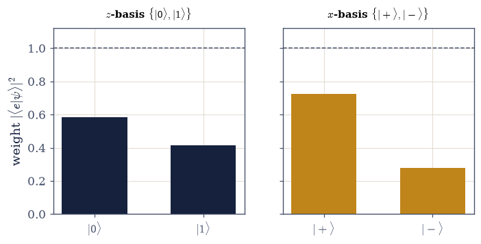
Fig. 513 One state, two bases, two sets of outcome-probabilities. The same qubit \(|\psi\rangle\) is resolved in the computational \(z\)-basis \(\{|0\rangle,|1\rangle\}\) (left, ink) and the \(x\)-basis \(\{|{+}\rangle,|{-}\rangle\}\) (right, amber); the bars are the projector weights \(|\langle e|\psi\rangle|^2\). In each basis the weights sum to one (dashed line) — the resolution of the identity guarantees it — yet the two distributions differ, because the bases ask different questions of the state. This is the whole content of measuring in different bases, here pure linear algebra; the physics of why these are probabilities is the Born rule (§6.5), and the geometry behind the two bases is the Bloch sphere (§6.8).

Exercise 8 — The calculus of states and operators (synthesis)

Dirac notation turned the inner product into a bra acting on a ket, the outer product into an operator, and three constructions into the working calculus of quantum mechanics. With the projector \(|e\rangle\langle e|\) we extract a component; with the resolution of the identity \(\sum_i|e_i\rangle\langle e_i|=I\) we expand in any basis at will — insert the identity; with the spectral decomposition \(A=\sum_i\lambda_i|\lambda_i\rangle\langle\lambda_i|\) we diagonalize; and with \(f(A)=\sum_i f(\lambda_i)|\lambda_i\rangle\langle\lambda_i|\) we apply any function to an operator by applying it to the eigenvalues. The arsenal is complete: we have the space (§6.1), the operators (§6.2), and now the language (§6.3). Movement 0 is closed.

There is no new computation to run: the calculus is the result. We have spent three notebooks building it and have not yet measured anything — and yet the apparatus of measurement is already in our hands. The projector we built is a measurement outcome; the resolution of the identity is the set of possible outcomes; the spectral decomposition is the observable, its eigenvalues the results and its projectors the outcomes. The physics was hiding in the notation. The next notebook (§6.4) lets it out, taking this entire apparatus to the Stern–Gerlach experiment and the two-state system — the first real measurement of the volume, and the start of Movement I.

Notebook summary

Dirac notation, the language of the rest of the volume, and the close of Movement 0.

• Kets, bras, the dual space Eq. 501: a ket is a state; a bra \(\langle\phi|=\)phi.conj() is the linear functional “inner product with \(\phi\)”; \(\langle\phi|\psi\rangle\) is a number.

• The outer product Eq. 502: \(|u\rangle\langle v|=\)numpy.outer(u, numpy.conj(v)) is an operator, \(\big(|u\rangle\langle v|\big)|w\rangle=\langle v|w\rangle|u\rangle\).

• Projectors Eq. 503: \(P=|e\rangle\langle e|\) is idempotent, Hermitian, rank-1, and extracts the \(e\)-component — the mathematics of a measurement (§6.5).

• The resolution of the identity Eq. 504: \(\sum_i|e_i\rangle\langle e_i|=I\) — insert the identity to expand in any basis; recovers the coefficients of §6.1 as projections.

• Change of basis Eq. 505: a unitary \(A'=U^{\dagger}AU\), \(\psi'=U^{\dagger}\psi\), preserving eigenvalues and inner products — a passive relabelling.

• The spectral decomposition Eq. 506: \(A=\sum_i\lambda_i|\lambda_i\rangle\langle \lambda_i|\), the eigen-projectors orthogonal and complete — “diagonalize” in its cleanest form.

• Functions of operators Eq. 507: \(f(A)=\sum_i f(\lambda_i)|\lambda_i\rangle \langle\lambda_i|\); \(e^{-iH}\) matches scipy.linalg.expm, the seed of time evolution (§6.7).

The arsenal is complete — the space, the operators, the language. The projector is already a measurement, the resolution of the identity already the set of outcomes, the spectral decomposition already the observable. The physics was hiding in the notation; Movement I lets it out.

Outlook

• The postulates of quantum mechanics (§6.5), written in this language: observables as Hermitian operators, outcomes as eigenvalues, probabilities as \(|\langle\lambda|\psi\rangle|^2\), measurement as projection.

• The Stern–Gerlach experiment and the two-state system (§6.4): the formalism meets a real measurement, and Movement I begins.

• The time-evolution operator (§6.7): \(U(t)=e^{-iHt/\hbar}=\sum_n e^{-iE_nt/\hbar}|n\rangle\langle n|\), the prime function of an operator.

• Cross-reference §6.1 (the inner product, expansion coefficients), §6.2 (the spectral theorem, the exponential map), and forward to §6.4, §6.5, §6.7, §6.8.

Take this notebook with you

Use the download button (↓) in the toolbar above to save this notebook and run it yourself. The published notebooks ship without worked solutions; if you would like the reference solutions — to teach from or to check your own work — get in touch: hello@ramador.me.