2.3 Hamiltonian Mechanics and Phase Flow

Elementary Computational Physics

Volume II — Analytical Mechanics Notebook 2.3

From the Lagrangian to phase space: the Legendre transform, Hamilton's equations, Poisson brackets, and Liouville's theorem — why a cloud of states flows like an incompressible fluid.

Level · intermediate   •   Est. · 75–100 min

Raymond Amador v1.4.0  ·  2026-07-31  ·  CC BY 4.0 (text) / MIT (code)

Notebook overview

§2.1 built mechanics out of a single scalar, the Lagrangian \(\mathcal L(q,\dot q,t)\), and the second-order Euler–Lagrange equations. Hamiltonian mechanics performs one more change of variables (trading the velocity \(\dot q\) for the conjugate momentum \(p = \partial\mathcal L/\partial\dot q\)) and in doing so flattens the dynamics into a beautifully symmetric set of first-order equations. The state of the system becomes a single point \((q,p)\) in phase space, and time evolution becomes a flow of that point along a vector field.

That geometric picture is the real payoff. Conserved quantities are functions that the flow leaves unchanged; symmetries and conservation laws are unified by the Poisson bracket; and the flow itself turns out to be incompressible: a cloud of initial conditions can shear and wind into the most intricate filament imaginable, but its phase-space volume never changes. That is Liouville’s theorem, and it is the exact statement behind a fact we already met empirically in §1.6: a symplectic integrator (velocity Verlet) kept energy bounded because it respected this area-preserving geometry. Here we see why.

We build a small toolkit (a symbolic Legendre transform, a hamilton_rhs that turns any \(H\) into an ODE right-hand side, and a symbolic Poisson bracket) and put it to work on the pendulum and the two-dimensional central force: deriving \(H\), reproducing the Lagrangian dynamics, drawing the classic pendulum phase portrait with its separatrix, checking conservation laws with brackets, distinguishing canonical from non-canonical transformations, and finally animating a phase-space ensemble to watch Liouville’s theorem hold.

How to read the checks. Each exercise ends with a validation that compares a computed result to an expected physical fact. A ✗ does not by itself mean the physics is wrong: it means the output didn’t match what the check expected, which may be a real error, a different-but-valid convention (a sign, a unit, an array order), or simply too tight a tolerance. Treat a ✗ as a prompt to locate the discrepancy; passing is strong evidence of correctness, not proof.

Scope. This is a working review, not a textbook chapter. For the canonical formalism in full (the Legendre transform, canonical transformations, Hamilton–Jacobi theory), see Nolting, Theoretical Physics 2 [Nol16], Goldstein, Poole & Safko [GPS02] (ch. 8–9), and Landau & Lifshitz, Mechanics [LL76].

Theory in brief

The Legendre transform: from \(\dot q\) to \(p\)

The conjugate momentum introduced in §2.1, restated as Eq. 143 below, is the gateway. Starting from \(\mathcal L(q,\dot q,t)\), define for each coordinate

(143)\[p_i = \frac{\partial \mathcal L}{\partial \dot q_i} ,\]

and pass to the Hamiltonian by the Legendre transform

(144)\[H(q,p,t) = \sum_i p_i\,\dot q_i - \mathcal L ,\]

in which every \(\dot q_i\) is re-expressed in terms of the momenta by inverting Eq. 143. When \(\mathcal L\) has no explicit time dependence and the constraints are scleronomic (time-independent), \(H\) equals the total energy \(T+V\), but its proper arguments are \((q,p)\), not \((q,\dot q)\).

Hamilton’s equations

Differentiating Eq. 144 and using Eq. 143 collapses the \(n\) second-order Euler–Lagrange equations into \(2n\) first-order ones,

(145)\[\dot q_i = \frac{\partial H}{\partial p_i} , \qquad \dot p_i = -\,\frac{\partial H}{\partial q_i} .\]

These are Hamilton’s equations. The system’s state is the point \((q,p)\in\mathbb R^{2n}\) of phase space, and Eq. 145 defines a velocity field on it; integrating the field is the phase flow.

Poisson brackets

For any two phase-space functions \(f(q,p)\) and \(g(q,p)\), the Poisson bracket is

(146)\[\{f,g\} = \sum_i \left( \frac{\partial f}{\partial q_i}\frac{\partial g}{\partial p_i} - \frac{\partial f}{\partial p_i}\frac{\partial g}{\partial q_i} \right) .\]

The total time derivative of any observable is then \(\mathrm df/\mathrm dt = \{f,H\} + \partial f/\partial t\), so a quantity with no explicit time dependence is conserved precisely when \(\{f,H\}=0\): the bracket form of the symmetry/conservation link of §2.2. The fundamental brackets \(\{q_i,p_j\}=\delta_{ij}\) are the fingerprint of canonical coordinates, and a change of variables is canonical exactly when it preserves them.

Liouville’s theorem

The phase-flow velocity field \((\dot q,\dot p)\) from Eq. 145 is divergence-free,

(147)\[\frac{\partial \dot q_i}{\partial q_i} + \frac{\partial \dot p_i}{\partial p_i} = \frac{\partial^2 H}{\partial q_i\,\partial p_i} - \frac{\partial^2 H}{\partial p_i\,\partial q_i} = 0 ,\]

so the flow is incompressible: a region of phase space is carried by the flow to a new region of exactly the same volume (Liouville’s theorem). This is the geometric reason a symplectic integrator conserves energy on average (§1.6), and it is the cornerstone of statistical mechanics: the conserved phase volume is what makes the microcanonical ensemble well defined (a forward link to Volume V).

---

Setup

Setup holds the toolchain — SymPy for the symbolic algebra, NumPy and SciPy to integrate Hamilton’s equations and evolve phase-space ensembles — the time symbol \(t\) of the Lagrangian picture, the euler_lagrange engine you built in §2.1 (imported from ecp.mechanics, used here only to cross-check), and one measuring instrument, shoelace_area. This notebook’s own machinery is not here: you write legendre_transform in Exercise 1, hamilton_rhs in Exercise 2, and the Poisson bracket poisson in Exercise 4, and the later exercises run on all three.

The Setup below holds this notebook’s data and instruments — nothing you are asked to build. It is collapsed so the building stays yours; expand it whenever you want the details.

Show code cell source

Hide code cell source

import numpy as np
import sympy as sp
from scipy.integrate import solve_ivp
import matplotlib.pyplot as plt
from matplotlib.animation import FuncAnimation

from ecp import draw, validate

# built from scratch in §2.1 (Exercise 1, certified on the harmonic oscillator);
# restated here as an instrument for the Lagrangian cross-check of Exercise 2.
from ecp.mechanics import euler_lagrange
from ecp.animate import show

# data: the time variable of the Lagrangian (velocity) picture
t = sp.symbols("t")


# instrument: a geometric measuring tape. The shoelace formula reads the area of
# an ordered polygon; the physics under test is that the flow preserves that
# area, not how the polygon is measured.
def shoelace_area(x, y):
    """Polygon area of an ordered closed vertex set (shoelace formula).

    Measures the phase-space area of a blob, the quantity Liouville's theorem conserves.

    Parameters
    ----------
    x, y : numpy.ndarray
        Ordered boundary vertices.

    Returns
    -------
    float
        The enclosed area.
    """
    return 0.5 * np.abs(np.dot(x, np.roll(y, -1)) - np.dot(y, np.roll(x, -1)))

Exercise 1 — Legendre-transform a Lagrangian into a Hamiltonian

The whole formalism begins with one change of variables. Given the pendulum Lagrangian Eq. 137-style scalar \(\mathcal L = \tfrac12 m\ell^2 \dot\theta^2 + mg\ell\cos\theta\), the conjugate momentum Eq. 143 is \(p_\theta = \partial\mathcal L/\partial\dot\theta = m\ell^2\dot\theta\), and the Legendre transform Eq. 144 produces \(H(\theta,p_\theta)\). Doing this by hand is a one-line calculation; doing it symbolically makes the recipe reusable, and the reusable version is what the rest of the notebook runs on. The pendulum is the right system to certify it against, because its answer is known cold: \(H = p_\theta^2/(2m\ell^2) - mg\ell\cos\theta\), the kinetic term inverting the moment of inertia \(m\ell^2\) and the potential carrying over from \(\mathcal L\) unchanged. The phase plane \((\theta, p_\theta)\) in which \(H\) lives is sketched in Fig. 124.

1. Write legendre_transform(L, qdots, ps): form the momentum definitions \(p_i = \partial\mathcal L/\partial\dot q_i\) of Eq. 143, solve them for the velocities (sympy.solve with dict=True), and substitute that map into \(H = \sum_i p_i\dot q_i - \mathcal L\) from Eq. 144, returning the simplified \(H(q,p)\) together with the velocity-to-momentum map. Write this one yourself — the implementation is the lesson.

2. Write \(\mathcal L\) for the pendulum in the velocity symbol \(\dot\theta\), and form \(p_\theta\) from Eq. 143 (sympy.diff).

3. Apply your engine to obtain \(H(\theta,p_\theta)\), and confirm it equals \(p_\theta^2/(2m\ell^2) - mg\ell\cos\theta\).

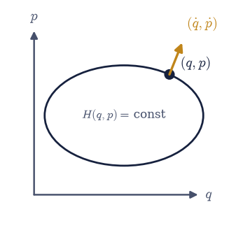
Fig. 124 The phase plane of a one-degree-of-freedom system: a state is a single point \((q,p)\) with \(q\) the generalized coordinate (horizontal) and \(p\) its conjugate momentum (vertical); under Hamilton’s equations the point flows along a curve of constant energy (the closed orbit shown), and the Hamiltonian \(H(q,p)\) is the conserved quantity labelling that curve.

conjugate momentum p_θ = l**2*m*thetadot
Hamiltonian H(θ, p_θ) = -g*l*m*cos(theta) + p_theta**2/(2*l**2*m)

Validation 1 — the pendulum Hamiltonian

The transform must return \(H = p_\theta^2/(2m\ell^2) - mg\ell\cos\theta\): the kinetic term inverts the moment of inertia \(m\ell^2\), and the potential \(-mg\ell\cos\theta\) carries over from \(\mathcal L\) with the sign it has in \(V = -mg\ell\cos\theta\).

✓  pendulum Hamiltonian is p_θ²/(2mℓ²) − mgℓcosθ

True

Exercise 2 — Hamilton’s equations reproduce the dynamics

A change of variables must not change the physics. Hamilton’s equations Eq. 145 for the pendulum read \(\dot\theta = \partial H/\partial p_\theta = p_\theta/(m\ell^2)\) and \(\dot p_\theta = -\partial H/\partial\theta = -mg\ell\sin\theta\): two first-order equations that must integrate to the same \(\theta(t)\) as the single second-order Euler–Lagrange equation \(\ddot\theta = -(g/\ell)\sin\theta\). We test exactly that, using the same physical pendulum sketched in Fig. 125. Getting there needs one more piece of machinery: something that takes any symbolic \(H\) and hands scipy.integrate.solve_ivp a numerical right-hand side. solve_ivp wants a first-order system, and Eq. 145 already is one, so the natural packaging is the block state \(y = [q_0,\dots,q_{n-1},p_0,\dots,p_{n-1}]\).

1. Write hamilton_rhs(H, qs, ps): differentiate \(H\) to get \(\partial H/\partial p_i\) and \(-\partial H/\partial q_i\) from Eq. 145, sympy.lambdify each one over the symbols \((q\dots,p\dots)\), and return a closure rhs(t, y) that evaluates them into the block state above. Write this one yourself — the implementation is the lesson.

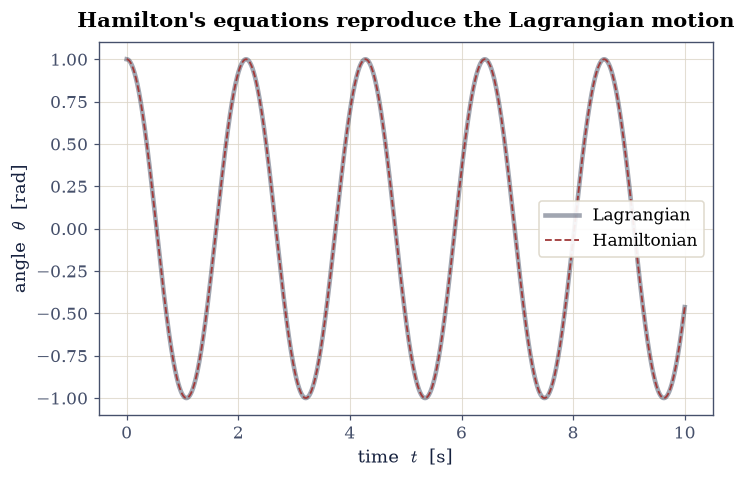
2. Build the numeric Hamiltonian (set \(m=\ell=1\), \(g=9.81\)), form the ODE right-hand side with your engine, and integrate it with scipy.integrate.solve_ivp (DOP853, rtol=1e-11, atol=1e-13) on a dense t_eval from \(\theta_0=1\) rad at rest (\(p_\theta=0\)).

3. Independently integrate the Lagrangian equation \(\ddot\theta=-(g/\ell)\sin\theta\) (derived with the euler_lagrange engine of §2.1, restated in Setup and integrated with the same solve_ivp/DOP853 settings) from the same initial state, and overlay the two \(\theta(t)\) curves.

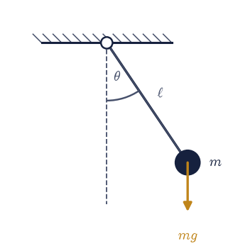
Fig. 125 The simple pendulum used to compare the two formalisms: a bob of mass \(m\) on a rigid rod of length \(\ell\) swings to angle \(\theta\) from the downward vertical (dashed) under gravity \(g\); its state is \((\theta,\dot\theta)\) in the Lagrangian picture and \((\theta,p_\theta)\) with \(p_\theta=m\ell^2\dot\theta\) in the Hamiltonian picture.

symbolic EL acceleration θ̈ = -9.81*sin(theta(t))

Validation 2 — same motion from both formalisms

The Hamiltonian and Lagrangian trajectories are the same physics expressed in different variables, so \(\theta(t)\) must agree pointwise to integration tolerance.

✓  Hamilton's equations give the same motion as the Lagrangian   [max|Δ| = 0 (rtol=1e-06, atol=1e-07)]

True

Exercise 3 — The phase portrait of the pendulum

Phase space lets us see all the motions at once. Because \(H\) is conserved along every trajectory (Eq. 145 implies \(\mathrm dH/\mathrm dt=0\) for an autonomous system), each trajectory is a level curve of \(H(\theta,p_\theta)\). The resulting phase portrait has three regimes separated by a critical curve, the separatrix at \(H = mg\ell\) (the energy of the upright equilibrium): closed librations (back-and-forth swinging) inside it, unbounded rotations (the bob going over the top) outside it, and the separatrix itself.

(A word on terminology: “libration” here is this small-oscillation, back-and-forth sense. The same word names the libration points of the restricted three-body problem, the classical name for the Lagrange points of §2.9, where a body librates around an equilibrium. The two senses are related but distinct, and we keep them separate.)

1. Integrate Hamilton’s equations (the hamilton_rhs you wrote in Exercise 2, with scipy.integrate.solve_ivp, DOP853) for several initial energies and plot the trajectories in the \((\theta, p_\theta)\) plane, densely sampled; overlay the level sets of \(H\) (matplotlib’s contour) and highlight the separatrix \(H=mg\ell\).

2. Confirm \(H\) is conserved along one trajectory using the series \(H(\theta(t), p_\theta(t))\).

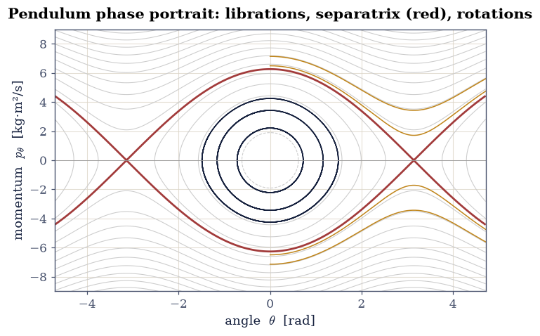
H relative drift along a libration = 4.05e-10

Validation 3 — energy is conserved along the flow

A phase trajectory is a level set of \(H\), so the numerically integrated \(H(\theta(t),p_\theta(t))\) must be constant to integration tolerance.

✓  H is conserved along a phase trajectory   [max relative drift = 2.37695e-10 (limit 1e-06)]

True

Exercise 4 — Poisson brackets and conservation

The Poisson bracket Eq. 146 turns “is this conserved?” into algebra: for an autonomous system, \(\mathrm df/\mathrm dt = \{f,H\}\), so \(f\) is conserved iff \(\{f,H\}=0\). Two facts follow immediately. First, \(\{H,H\}=0\), so energy is always conserved. Second, reconnecting to Noether’s theorem (§2.2), for a two-dimensional central potential \(H = (p_x^2+p_y^2)/2m + V(r)\) with \(r=\sqrt{x^2+y^2}\), the angular momentum \(L_z = x p_y - y p_x\) satisfies \(\{L_z,H\}=0\): rotational symmetry, now read straight off the bracket.

1. Write poisson(f, g, qs, ps), the symbolic bracket Eq. 146: sum \(\partial f/\partial q_i\,\partial g/\partial p_i - \partial f/\partial p_i\,\partial g/\partial q_i\) over the conjugate pairs (sympy.diff). Write this one yourself — the implementation is the lesson.

2. Use it to confirm \(\{H,H\}=0\) for the central-force Hamiltonian.

3. Form \(L_z = x p_y - y p_x\) and confirm \(\{L_z,H\}=0\), so angular momentum is conserved.

{H, H}   = 0
{L_z, H} = 0

Validation 4 — angular momentum is conserved

Both brackets must vanish identically: \(\{H,H\}=0\) trivially, and \(\{L_z,H\}=0\) because the central potential is rotationally invariant.

✓  {H, H} = 0 (energy is conserved)
✓  {L_z, H} = 0 ⇒ angular momentum conserved (central force)

True

Exercise 5 — Canonical transformations preserve the bracket

Not every change of phase-space variables is legal. A transformation \((q,p)\mapsto(Q,P)\) is canonical (it preserves the form of Hamilton’s equations) exactly when it preserves the fundamental bracket, \(\{Q,P\}=1\) (Eq. 146). A rotation in the \((q,p)\) plane, \(Q = q\cos\alpha - p\sin\alpha\), \(P = q\sin\alpha + p\cos\alpha\), passes; a naive rescaling \(Q=q,\ P=2p\) does not. This is the same contrast as the symmetry-versus-broken-symmetry of §2.2: preserving the bracket is the structural test.

1. Show the phase-plane rotation has \(\{Q,P\}=1\) for arbitrary angle \(\alpha\) (your Exercise 4 poisson, with sympy.simplify).

2. Show the rescaling \(Q=q,\ P=2p\) gives \(\{Q,P\}=2\neq1\), so it is not canonical.

rotation:  {Q, P} = 1
rescaling: {Q, P} = 2

Validation 5 — only the bracket-preserving map is canonical

The rotation must give \(\{Q,P\}=1\) for every \(\alpha\) (canonical); the rescaling must give \(\{Q,P\}=2\neq1\) (not canonical).

✓  the phase-plane rotation is a canonical transformation
✓  the rescaling Q=q, P=2p is NOT canonical ({Q,P}=2≠1)

True

Exercise 6 — Liouville’s theorem: area is preserved as the blob shears (worked animation)

Here is the geometric heart of the subject, made visible. Take a whole cloud of initial conditions (a lumpy closed ring of a few hundred points bounding a blob in the phase plane) and evolve every point under Hamilton’s flow Eq. 145. The lesson of Liouville’s theorem Eq. 147 is subtle, so the choice of system matters. For the harmonic oscillator the flow is a rigid rotation, and a blob would merely turn without changing shape: area-preservation would hold trivially, inviting the wrong inference that the area is fixed because the shape is rigid. It is not. We use the pendulum instead, whose libration period grows with amplitude: a blob spanning a range of energies then shears (its lower-energy edge advancing faster than its higher-energy edge) stretching and curling into an amoeba. Liouville’s theorem says the enclosed area stays exactly constant despite that distortion. That is the non-trivial content, and the reason to switch flows.

We keep the blob well inside the libration region, away from the separatrix, so it distorts moderately (an amoeba, still a simple closed curve) rather than filamenting: Exercise 7 then pushes the very same mechanism to the extreme across the separatrix. The two are stages of one phenomenon: moderate shear here, runaway shear there.

This is the same area-preservation we measured for velocity Verlet in §1.6, and now we can say why it mattered: Verlet’s discrete update is itself a canonical map, so it inherits this incompressibility and cannot let the energy drift away. This is the worked animation; you build the second in Exercise 7. The animation shows the blob shearing; the validation measures its enclosed area, not the animation object. (Note: as the blob shears, its boundary points spread unevenly (that non-uniform spacing is the shear), so we track a finely resolved ring to keep the polygon-area measurement faithful, and judge it against an honest tolerance for a sheared finite-point boundary, not machine zero.)

pendulum blob area: 0.6497 → 0.6497 (relative drift 3.4e-06)

Once Loop Reflect

Fig. 126 Animation of a phase-space blob evolving under the pendulum’s Hamiltonian flow, well inside the libration region (separatrix dashed, \(p=\pm2\cos(\theta/2)\)): because the libration period grows with amplitude, the blob shears — its lower-energy edge outrunning its higher-energy edge — and curls into an amoeba, yet its enclosed area (shaded) stays constant. That invariance under distortion is the non-trivial content of Liouville’s theorem; here \(q=\theta\) and \(p\) is its conjugate momentum.

Validation 6 — the area is invariant despite the shear

Liouville’s theorem Eq. 147 demands the enclosed area stay constant as the ensemble flows and shears. The check reads the polygon area of the animated blob at every frame, so it validates the physics on screen rather than the FuncAnimation object. The tolerance is set for a sheared, finite-point boundary: the dynamics conserves area exactly, but the shoelace measurement of a stretching polygon does not, so a few percent is honest here (cf. the discretization theme of §0.1), not the machine-zero of an analytic invariant.

✓  phase-space area is preserved as the blob shears (Liouville)   [max relative drift = 3.40614e-06 (limit 0.02)]

True

Exercise 7 — Mixing near the separatrix (student-implemented animation)

Liouville’s theorem says the area is preserved: it says nothing about the shape. Near the pendulum separatrix, points just inside librate while points just outside rotate, so a compact blob is sheared into an ever-thinner filament that winds around the phase plane. The area is unchanged, but the shape becomes arbitrarily intricate. This stretching-and-folding is the seed of chaos and ergodicity, and the reason a Hamiltonian system explores its energy surface: the microscopic basis of statistical mechanics (a forward link to Volume V).

This is the student-implemented animation: the dynamics and the evolved ensemble are prepared for you; you build the player. The validation checks the physics of the animated data: that the area is still conserved despite the dramatic distortion.

1. Evolve a small ring of initial conditions straddling the pendulum separatrix under the flow \(\dot\theta = p_\theta,\ \dot p_\theta = -\sin\theta\) (unit pendulum) with scipy.integrate.solve_ivp (DOP853), storing every frame.

2. Build the animation of the filamenting ensemble over the phase plane — there are many valid ways to draw it — then plt.close(fig) and end with ecp.animate.show(anim).

3. Confirm the enclosed area (the shoelace_area helper) is still conserved as the blob filaments.

A ✗ on the final check is about the area measurement or the ensemble we evolved, not the drawing: any correct animation of the same data is fine. If it fails, check that the ring stays well resolved (enough boundary points) and that the shoelace area uses the ordered ring.

pendulum blob area: 0.3848 → 0.3850 (relative drift 3.1e-04)

Once Loop Reflect

Fig. 127 Animation of a phase-space blob straddling the pendulum separatrix (grey, \(p=\pm2\cos(\theta/2)\)): points inside librate and points outside rotate, so the initially circular ring (blue) is sheared into a thin winding filament; its enclosed area is nonetheless conserved, the area-preserving mixing that underlies ergodicity and statistical mechanics.

Validation 7 — area survives the filamentation

Even as the ensemble winds into a thin filament, Liouville’s theorem Eq. 147 keeps its area fixed. The check measures the polygon area of the (still ordered) ring across the run.

✓  area is preserved even as the ensemble filaments near the separatrix   [max relative drift = 0.000301845 (limit 0.01)]

True

Notebook summary

• The Legendre transform \(L\to H\) and Hamilton’s equations reproducing the dynamics (the legendre_transform and hamilton_rhs you wrote, available to the rest of the series as ecp.mechanics.hamilton_rhs); the pendulum’s phase portrait with its separatrix.

• Poisson brackets as the algebra of conservation (\(\{H,H\}=0\), \(\{L_z,H\}=0\) for a central force); canonical transformations preserving the bracket (a phase-plane rotation is canonical, the rescaling \(Q=q,P=2p\) is not, \(\{Q,P\}=2\)).

• Liouville’s theorem: a phase-space blob shears but conserves its area, and mixing near the separatrix.

Outlook

• Action–angle variables. For the pendulum’s librations one can change to coordinates \((\,I,\phi\,)\) in which \(I=\oint p\,\mathrm dq/2\pi\) is constant and \(\phi\) advances linearly: the natural language for adiabatic invariants and perturbation theory.

• The flow as a symplectic map. The time-\(\tau\) phase flow is a canonical map with unit Jacobian determinant; this is the rigorous statement behind the measurement of §1.6 that velocity Verlet has \(\det = 1\).

• Hamilton–Jacobi. Seeking a canonical transformation that makes \(H\) vanish leads to the Hamilton–Jacobi equation, whose action \(S\) plays the role of a wave’s phase: the bridge to the eikonal/quantum analogy in Volume VI.

• Toward statistical mechanics. Liouville’s theorem makes the phase-space measure invariant, which is exactly what a microcanonical ensemble needs to be well defined: the entry point to Volume V.

References

[GPS02]

Herbert Goldstein, Charles P. Poole, and John L. Safko. Classical Mechanics. Pearson, 3 edition, 2002.

[LL76]

L. D. Landau and E. M. Lifshitz. Mechanics. Volume 1 of Course of Theoretical Physics. Butterworth–Heinemann, 3 edition, 1976.

[Nol16]

Wolfgang Nolting. Theoretical Physics 2: Analytical Mechanics. Springer, 2016.

Take this notebook with you

Use the download button (↓) in the toolbar above to save this notebook and run it yourself. The published notebooks ship without worked solutions; if you would like the reference solutions — to teach from or to check your own work — get in touch: hello@ramador.me.