


3.9 Waveguides and Cavity Resonances#
Notebook overview#
The free plane wave of §3.8 could take any frequency and travel in any direction. Put it inside a hollow metal pipe and everything changes: the conducting walls force boundary conditions on the field, and only a discrete set of transverse patterns, the modes, can propagate, each with its own cutoff frequency below which it simply will not go. Close the pipe at both ends and even the frequencies become discrete: the box rings only at its resonances. Confinement quantizes.
This notebook is a convergence of three threads the course has been building. The wave equation restricted to a cross-section is a Helmholtz eigenvalue problem; solving it is exactly the boundary-value problem of §3.4 (the discretized Laplacian), read as the eigenvalue problem of §0.5, giving the normal modes of §2.7, now for electromagnetic fields. We solve it twice: analytically for the separable rectangular guide, where the modes are products of sines and cosines, and numerically with a sparse eigensolver on the discretized cross-section, which also cracks shapes no separation of variables can touch.
The running example is the standard WR-90 X-band guide (\(a=22.9\,\)mm, \(b=10.2\,\)mm). We find its mode patterns and cutoffs, watch a mode switch from evanescent to propagating as the frequency crosses cutoff, recover the cutoffs from a sparse eigenproblem, take that solver to a non-separable cross-section, and finally close the guide into a 3-D cavity with discrete resonances. Throughout runs one parallel: the rectangular-guide eigenproblem is the same mathematics as a vibrating drumhead, and the cavity the same as a 3-D box, the classical rehearsal for the quantum particle in a box (Vol VI).
Everything is in SI units, with \(c=1/\sqrt{\mu_0\varepsilon_0}\). A guided wave does propagate, so exactly one figure here is animated, the dominant mode travelling down the guide; everything else is a still.
How to read the checks. Each exercise ends with a
validatecall against an independent fact: a sine mode satisfying the transverse Helmholtz equation, the dominant cutoff equal to \(c/2a\), a sparse eigensolver recovering the analytic cutoffs, a cavity resonance matching the box formula. A ✓ is strong evidence; a ✗ is a prompt to locate the discrepancy, not a verdict.A resolution note. The sparse cross-section eigensolver recovers the low-order cutoffs to about 0.1%, but the high-order modes drift downward: the five-point Dirichlet Laplacian under-estimates eigenvalues, and a fixed grid under-resolves their finer structure (too few nodes per half-wavelength). We validate on the well-resolved low modes and read the drift as the resolution lesson it is, the same honesty applied to the §3.4 corner and the §3.6 \(\nabla\cdot\mathbf B\) residual.
Theory in brief#
Confining a wave#
Inside a hollow perfect conductor the field still obeys the vacuum wave equation of §3.8, but now with the boundary condition that the tangential electric field vanishes on the walls. Seeking solutions that propagate along the guide axis \(\hat{\mathbf z}\) and keep a fixed transverse shape,
separates the problem: the transverse pattern \(\psi(x,y)\) obeys the Helmholtz equation \(\nabla_T^2\psi+k_c^2\psi=0\) on the cross-section, with \(k_c\) a separation constant fixed by the boundary.
TE and TM modes#
The guided fields split into two families: transverse electric (TE, \(E_z=0\)) and transverse magnetic (TM, \(B_z=0\)); Jackson, Classical Electrodynamics, ch. 8, carries the reduction of Maxwell’s equations to these two families out in full. For a rectangular guide \(a\times b\) the patterns are products of sines and cosines; the TM modes, with \(E_z=0\) on the walls, are
with integers \((m,n)\) labelling the mode (TE modes use cosines, the Neumann partner).
Cutoff frequency#
Substituting the travelling form Eq. 238 into the wave equation ties frequency and propagation constant to the separation constant, \((\omega/c)^2=\beta^2+k_c^2\); each mode therefore has a cutoff frequency
When \(\omega/c>k_c\) the propagation constant \(\beta\) is real and the mode travels with guide wavelength \(\lambda_g=2\pi/\beta>\lambda_{\mathrm{free}}\). When \(\omega/c<k_c\), \(\beta\) is imaginary: the mode is evanescent, decaying as \(e^{-\alpha z}\) with \(\alpha=\sqrt{k_c^2-(\omega/c)^2}\), and carries no power. The mode of lowest cutoff (the dominant mode, TE\(_{10}\) for a rectangular guide, \(f_c=c/2a\)) sets the single-mode band over which a guide is normally used.
The eigenvalue connection#
The transverse Helmholtz problem is an eigenvalue problem for the boundary-constrained Laplacian,
its eigenvalues the squared cutoffs \(k_c^2\) and its eigenvectors the mode patterns. This unifies three earlier ideas: the discretized Laplacian of the §3.4 boundary-value problem, the eigenvalue machinery of §0.5, and the normal modes of §2.7. We solve it analytically for the separable rectangle and numerically with a sparse eigensolver, which then handles cross-sections that do not separate.
Cavity resonances#
Cap the guide at both ends (\(z=0\) and \(z=d\)) and the field is confined in all three directions; only a discrete set of standing-wave frequencies survives,
These are the resonances of a microwave cavity, and the same box eigenproblem that, in Vol VI, sets the energy levels of a quantum particle in a box.
The drumhead parallel#
None of this is special to electromagnetism. The rectangular-guide eigenproblem is mathematically identical to a vibrating rectangular membrane (a 2-D box Helmholtz problem), and the cavity to a 3-D box. Confinement produces discrete modes is a universal theme, the same one met for coupled oscillators in §2.7 and waiting in the quantum bound states of Vol VI.
Setup#
Data and instruments only. The data are the CODATA constants that fix \(c\), the WR-90
cross-section, the series palette, and the closed forms the theory section has already
displayed: the squared cutoff wavenumber and the cutoff frequency Eq. 239,
Eq. 240, the sine and cosine mode patterns of the separable rectangle, and the
cavity resonance Eq. 242. Each of those functions is one line transcribed from
an equation above, the specimen the problem hands you rather than machinery anyone
builds. This notebook’s own machinery is not here: you write the sparse Dirichlet
transverse Laplacian neg_laplacian in Exercise 4, and every numerical mode that
follows is one of its eigenvectors, including the non-separable L-guide of Exercise 5
and the drumhead of Exercise 7. No randomness appears anywhere in this notebook.
The Setup below holds this notebook’s data and instruments — nothing you are asked to build. It is collapsed so the building stays yours; expand it whenever you want the details.
Exercise 1 — The rectangular waveguide and its modes (worked)#
A hollow rectangular pipe of width \(a\) and height \(b\) is the workhorse of microwave engineering. Inside it the transverse field of a TM\(_{mn}\) mode is the sine product Eq. 239, \(\psi\propto\sin(m\pi x/a)\sin(n\pi y/b)\), which vanishes on every wall and so satisfies the perfect-conductor boundary condition, with squared cutoff \(k_c^2=(m\pi/a)^2+(n\pi/b)^2\) (Fig. 263). We use the standard WR-90 X-band guide, \(a=22.9\,\)mm and \(b=10.2\,\)mm.
Evaluate the mode patterns on the cross-section grid and confirm numerically that a sine mode satisfies the transverse Helmholtz equation \(\nabla_T^2\psi=-k_c^2\psi\): apply the 5-point Laplacian (the §3.4 stencil) to the sampled \(\psi\) and compare to \(-k_c^2\psi\) on the interior, away from the wall nodes where the one-sided stencil is inexact.
Draw the transverse patterns of the lowest modes (Fig. 264) — the familiar half-wave humps of a constrained membrane.
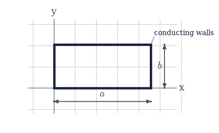
Fig. 263 The rectangular waveguide cross-section (WR-90: width \(a=22.9\,\)mm, height \(b=10.2\,\)mm), with the conducting walls (dark) on which the tangential electric field vanishes. The mode indices \((m,n)\) count the half-wavelengths of the field pattern across the width and height; the dominant TE\(_{10}\) mode has a single half-wave across \(a\) and none across \(b\).#
TM11: k_c² = 113684.0 m⁻², cutoff = 16.088 GHz
max relative |∇²ψ + k_c²ψ| on the interior = 5.08e-05
Validation 1#
✓ the sine-product mode satisfies the transverse Helmholtz equation ∇²ψ = −k_c²ψ
True
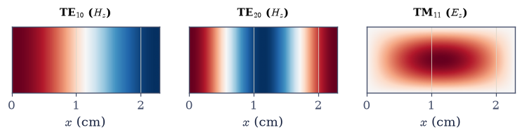
Fig. 264 Transverse mode patterns of the WR-90 guide: the TE\(_{10}\) and TE\(_{20}\) longitudinal magnetic field \(H_z\) (cosine products) and the TM\(_{11}\) longitudinal electric field \(E_z\) (a sine product, vanishing on the walls). Red and blue are opposite signs of the field; the indices \((m,n)\) count the half-waves across width and height. These are the same humped shapes a clamped membrane would take.#
Exercise 2 — Cutoff frequencies and the dominant mode (worked)#
Each mode carries a cutoff frequency \(f_c=c\,k_c/2\pi\) Eq. 240 below which it cannot propagate. The mode with the lowest cutoff is the dominant mode; for a rectangular guide with \(a>b\) that is TE\(_{10}\), whose cutoff is simply \(f_c=c/2a\). The band between the dominant cutoff and the next mode’s is the single-mode band, where only one pattern propagates and the guide is normally operated. The six modes surveyed below are \((1,0)\), \((2,0)\), \((0,1)\), \((1,1)\), \((3,0)\) and \((2,1)\); \(m=n=0\) is left out because it carries no transverse field.
Compute \(f_c\) Eq. 240 for those low modes.
Confirm the dominant-mode cutoff equals \(c/2a\).
Order the modes by cutoff and read off the single-mode band (Fig. 265).
mode (1, 0): f_c = 6.546 GHz
mode (2, 0): f_c = 13.091 GHz
mode (0, 1): f_c = 14.696 GHz
mode (1, 1): f_c = 16.088 GHz
mode (3, 0): f_c = 19.637 GHz
mode (2, 1): f_c = 19.681 GHz
dominant mode (1, 0): f_c = 6.546 GHz (c/2a = 6.546 GHz)
single-mode band: 6.55–13.09 GHz
Validation 2#
✓ the dominant-mode cutoff is c/(2a) (TE10) [got 6.54569e+09 vs expected 6.54569e+09 (rtol=1e-06, atol=1e-09)]
✓ the modes order by cutoff with TE10 dominant and TE20 next
True
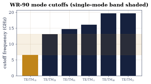
Fig. 265 Cutoff frequencies of the low WR-90 modes, ordered low to high. The dominant TE\(_{10}\) mode (amber) sits at \(c/2a=6.55\,\)GHz; the shaded band up to TE\(_{20}\) at \(13.1\,\)GHz is the single-mode range, where only TE\(_{10}\) propagates and the guide carries a clean signal. Above it, higher modes switch on one by one.#
Exercise 3 — Evanescent versus propagating (worked)#
Whether a mode travels depends entirely on how its drive frequency compares to its cutoff. The guide propagation constant is \(\beta=\sqrt{(\omega/c)^2-k_c^2}\) Eq. 240. Above cutoff \(\beta\) is real and the mode propagates with guide wavelength \(\lambda_g=2\pi/\beta\); below cutoff the quantity under the root is negative, \(\beta\) is imaginary, and the mode is evanescent, dying away as \(e^{-\alpha z}\) with \(\alpha=\sqrt{k_c^2-(\omega/c)^2}\). The mode probed here is the dominant TE\(_{10}\), whose cutoff Exercise 2 put at \(f_c=6.55\,\)GHz, so the three drive frequencies \(6\), \(8\) and \(12\,\)GHz straddle it: one below, two above. The animation (Fig. 267) then shows that mode travelling down the guide above cutoff, the wave the whole device exists to carry.
Evaluate \(\beta\) at \(6\), \(8\), and \(12\,\)GHz.
Confirm the mode is evanescent below cutoff, with decay rate \(\alpha\), and propagating above (Fig. 266).
6 GHz: evanescent, α = 54.8 /m
8 GHz: propagating, β = 96.4 /m, λ_g = 65.2 mm
12 GHz: propagating, β = 210.8 /m, λ_g = 29.8 mm
Validation 3#
✓ below cutoff the mode is evanescent (β imaginary); above cutoff it propagates
True
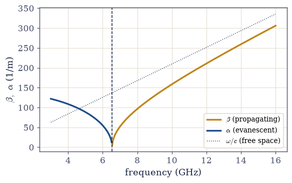
Fig. 266 Guide dispersion of the TE\(_{10}\) mode: the propagation constant \(\beta\) (amber, above cutoff) and the evanescent decay rate \(\alpha\) (blue, below cutoff) against frequency, with the cutoff \(f_c=6.55\,\)GHz marked. The mode does not propagate at all below cutoff; just above it \(\beta\) rises steeply from zero, and far above it approaches the free-space \(\omega/c\) (dotted).#
Fig. 267 Animation of the dominant TE\(_{10}\) mode propagating along the WR-90 guide at \(10\,\)GHz (above cutoff). The colour is the transverse electric field \(E_y=E_0\sin(\pi x/a)\cos(\beta z-\omega t)\) in a top-view \(x\)–\(z\) slice: a single half-wave hump across the width \(a\), the whole pattern marching down the guide at the phase velocity \(\omega/\beta\). One guide wavelength \(\lambda_g=2\pi/\beta\) spans one full colour cycle along \(z\).#
Exercise 4 — The eigenvalue problem, numerically (worked)#
Here the threads converge. The transverse Helmholtz problem Eq. 241 is an eigenvalue problem for the boundary-constrained Laplacian: discretize \(-\nabla_T^2\) on the cross-section with the §3.4 five-point stencil and Dirichlet walls, and its eigenvalues are the squared cutoffs \(k_c^2\), its eigenvectors the TM mode patterns. This is the §3.4 boundary-value problem solved as the §0.5 eigenproblem, giving the §2.7 normal modes, now for fields.
The matrix is the one §3.4 assembled for the square box, generalized in the two ways the rest of this notebook needs. It takes separate spacings \(h_x\neq h_y\), because a waveguide cross-section is not square, and it takes a boolean mask of interior nodes, so that the very same builder serves the rectangle here and the L-shape of Exercise 5. With the walls grounded there is no right-hand side to fold the boundary into: a neighbour outside the mask simply contributes nothing, which is the perfect-conductor Dirichlet condition written as an omission. Since the operator is wanted itself rather than a solution of it, the builder returns the matrix together with the map from grid position to row index, the bookkeeping that lets an eigenvector be scattered back onto the grid as a picture.
Write
neg_laplacian(mask, hx, hy), the sparse \(-\nabla_T^2\) over theTruenodes ofmask(indexedmask[j, i], withjrunning over \(y\)): number those nodes, give each its own row with \(2/h_x^2+2/h_y^2\) on the diagonal and \(-1/h^2\) in the column of every in-mask neighbour, and return the matrix and the index map. Write this one yourself — the implementation is the lesson: this matrix is the confined wave equation Eq. 241, and every numerical mode in the rest of the notebook is one of its eigenvectors.Assemble it on an \(N_x\times N_y\) interior grid of the WR-90 rectangle and solve for the lowest eigenvalues with
scipy.sparse.linalg.eigsh(shift-invert about zero for the smallest).Compare the numerical \(k_c^2\) to the analytic TM cutoffs for the low modes (Fig. 268); the higher modes drift downward because the five-point Dirichlet Laplacian under-estimates eigenvalues and the fixed grid under-resolves their finer structure — a resolution effect, not an error in the physics.
numerical k_c² analytic k_c² rel. error
113613.5 113684.0 0.06%
170029.9 170145.1 0.07%
263937.9 264247.1 0.12%
395158.8 395989.9 0.21%
397193.0 398274.6 0.27%
453609.4 454735.8 0.25%
low-mode (first three) max relative error = 0.12%
Validation 4#
✓ the sparse eigensolver recovers the analytic TM cutoffs for the low modes [max|Δ| = 309.198 (rtol=0.02, atol=1e-09)]
True
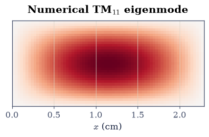
Fig. 268 The fundamental TM\(_{11}\) mode of the WR-90 guide, computed numerically as the lowest eigenvector of the discretized Dirichlet Laplacian (scipy.sparse.linalg.eigsh). It reproduces the analytic \(\sin(\pi x/a)\sin(\pi y/b)\) sine-product pattern to plotting accuracy: the eigenproblem of §0.5, applied to the boundary-value problem of §3.4, returns the waveguide mode of textbook theory.#
Exercise 5 — A non-separable cross-section (student)#
The analytic sine products work only because the rectangle separates. Real guides come
in shapes that do not, and there the numerical eigensolver earns its keep. Consider an
L-shaped cross-section, a square with one quadrant removed
(Fig. 269): there is no closed-form mode, but the same sparse Dirichlet
Laplacian gives its cutoffs and patterns directly. This is what the mask argument of
your Exercise 4 neg_laplacian was for: nothing about the builder changes, only which
nodes are marked True. The shape here is a \(20\,\)mm square with the top-right
quadrant removed, and its fundamental mode concentrates in the body of the L, avoiding
the re-entrant corner.
Build the L-shaped mask on the grid and assemble the
neg_laplacianyou wrote in Exercise 4 over it.Solve for the lowest modes with
scipy.sparse.linalg.eigsh.With no closed form to check against, validate by self-consistency: every eigenpair satisfies the discretized Helmholtz problem \(A\psi=k_c^2\psi\) to machine precision, and the lowest cutoff is real and positive.
L-shape lowest k_c² = 96568.0 m⁻² (f_c = 14.83 GHz)
eigenpair residual |Aψ − k_c²ψ| = 1.29e-09
Validation 5#
✓ the numerical eigensolver gives self-consistent modes of the non-separable L-guide
True
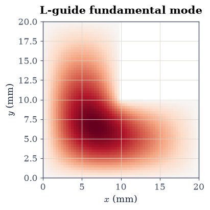
Fig. 269 The fundamental mode of an L-shaped guide (a \(20\,\)mm square with the top-right quarter removed, the white region outside the guide), from the sparse Dirichlet eigensolver. The field is a single smooth hump that fills the body of the L and is pulled away from the re-entrant corner. No separation of variables produces this pattern; the finite-difference eigenproblem gives it with the same code that solved the rectangle.#
Exercise 6 — Cavity resonances (worked)#
Cap the guide at both ends and the wave is trapped in all three directions. Only standing waves that fit the box survive, at the discrete resonant frequencies \(f_{mnp}=\tfrac{c}{2}\sqrt{(m/a)^2+(n/b)^2+(p/d)^2}\) Eq. 242 (Fig. 270). A microwave cavity is exactly this: a resonator that rings only at its eigenfrequencies, the electromagnetic cousin of an organ pipe. The cavity here is the WR-90 cross-section (\(a=22.9\,\)mm, \(b=10.2\,\)mm) closed at a length \(d=30\,\)mm. A triple \((m,n,p)\) with two zero indices carries an identically zero field, so only triples with at least two nonzero indices are modes. These discrete frequencies from 3-D confinement are the direct classical ancestor of the quantized energies of a quantum particle in a box (Vol VI), the very same eigenproblem.
Compute the low resonances \(f_{mnp}\) Eq. 242 of that cavity.
Confirm the lowest of them matches the box formula built directly from \(a\) and \(d\).
cavity mode (1, 0, 1): f = 8.235 GHz
cavity mode (1, 0, 2): f = 11.946 GHz
cavity mode (0, 1, 1): f = 15.522 GHz
cavity mode (1, 1, 0): f = 16.088 GHz
cavity mode (1, 1, 1): f = 16.846 GHz
TE101 resonance = 8.2348 GHz
Validation 6#
✓ the cavity resonance f_101 matches the box formula [got 8.23477e+09 vs expected 8.23477e+09 (rtol=1e-06, atol=1e-09)]
True
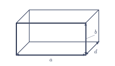
Fig. 270 A rectangular microwave cavity (\(a\times b\times d\)), a length of waveguide closed by conducting end walls, shown in oblique view. Trapped in all three directions, the field can only stand at the discrete resonances \(f_{mnp}=\tfrac{c}{2}\sqrt{(m/a)^2+(n/b)^2+(p/d)^2}\); the indices count half-waves along each edge. This is the 3-D box whose eigenproblem returns, unchanged, as the quantum particle in a box.#
Exercise 7 — The drumhead parallel (student)#
Nothing in Exercise 4 was about electromagnetism. The transverse Helmholtz eigenproblem \(-\nabla_T^2\psi=k_c^2\psi\) on a box, with \(\psi=0\) on the boundary, is identically the equation for the small vibrations of a clamped rectangular membrane, a drumhead, whose eigenvalues are its squared vibration frequencies (up to the wave speed) and whose eigenvectors are its mode shapes. The waveguide and the drum are the same problem (callback to the normal modes of §2.7). The match is exact in form, and confinement gives discrete modes whatever the field. The membrane here is \(30\times20\,\)mm, a shape no waveguide in this notebook has, which is the point: the agreement is not a coincidence of dimensions.
Solve the 2-D box Helmholtz eigenproblem on that membrane with the
neg_laplacianyou wrote in Exercise 4 and the same sparse eigensolver.Read the result as a vibrating drumhead: confirm its eigenvalues are the rectangular-guide cutoffs \(k_c^2=(m\pi/a)^2+(n\pi/b)^2\).
membrane k² = 35625.1 guide k_c² = 35640.2 (0.04%)
membrane k² = 68486.2 guide k_c² = 68538.9 (0.08%)
membrane k² = 109457.0 guide k_c² = 109662.3 (0.19%)
membrane k² = 123154.6 guide k_c² = 123370.1 (0.17%)
Validation 7#
✓ the drumhead modes are the same eigenproblem as the waveguide TM modes [max|Δ| = 205.274 (rtol=0.02, atol=1e-09)]
True
Exercise 8 — Confinement quantizes#
Step back from the machinery to the idea it keeps returning. A wave in open space is free: any frequency, any direction. The instant we wall it in, that freedom collapses into a discrete spectrum, a countable list of modes each with a cutoff, or, for a fully closed cavity, a countable list of resonant frequencies. The geometry alone selects which waves may exist. We met the selection three ways here and they were one thing: the boundary-value problem of §3.4, the eigenvalue problem of §0.5, and the normal modes of §2.7, all the statement \(-\nabla^2\psi=k^2\psi\) with \(\psi\) vanishing on the walls.
That is the classical rehearsal for the central fact of the quantum world. Replace the electromagnetic wave by a matter wave and the conducting box by a potential well, and the identical eigenproblem returns as the quantized energies of a particle in a box (Vol VI). The discreteness that seems so strange in quantum mechanics is, in its mathematics, nothing more exotic than a wave in a box, which we can see and compute here.
Two measured identities make that unification concrete one last time.
The lowest membrane eigenvalue of Exercise 7 equals its analytic \(k^2\) — the drumhead is the waveguide eigenproblem.
The cavity resonance of Exercise 6 decomposes into guide physics: \(f_{101}^2 = f_c(\mathrm{TE}_{10})^2 + (c/2d)^2\), the transverse cutoff of Exercise 2 plus a longitudinal half-wave — a 3-D resonance is a guided mode standing between the end walls.
membrane fundamental matches analytic k²: True
f_101 = 8.2348 GHz vs sqrt(f_c(TE10)² + (c/2d)²) = 8.2348 GHz (rel. diff 1.11e-16)
confinement → a discrete mode spectrum: the classical seed of quantization
Validation 8#
✓ confinement quantizes: the drumhead matches the guide eigenproblem, and the cavity resonance decomposes into guide cutoff + longitudinal half-wave
True
Notebook summary#
A hollow conductor turns the wave equation into a transverse Helmholtz eigenvalue problem Eq. 241; the rectangular guide’s TM modes are sine products \(\sin(m\pi x/a)\sin(n\pi y/b)\) with \(k_c^2=(m\pi/a)^2+(n\pi/b)^2\), verified to satisfy \(\nabla_T^2\psi=-k_c^2\psi\).
Cutoffs \(f_c=c\,k_c/2\pi\): the dominant WR-90 mode is TE\(_{10}\) at \(c/2a=6.55\,\)GHz, setting the single-mode band up to TE\(_{20}\) at \(13.1\,\)GHz. Below cutoff a mode is evanescent (\(\alpha=55\,\)/m at \(6\,\)GHz); above it propagates (\(\beta=96\,\)/m at \(8\,\)GHz), with the dominant mode animated travelling down the guide.
A sparse Dirichlet Laplacian +
scipy.sparse.linalg.eigshrecovers the analytic cutoffs for the low modes (to a couple of percent on this grid, the high modes drifting as resolution falls behind their structure), and it cracks a non-separable L-shaped guide that no sine product can.Closing the guide gives a 3-D cavity with discrete resonances \(f_{mnp}=\tfrac{c}{2} \sqrt{(m/a)^2+(n/b)^2+(p/d)^2}\); the drumhead carries the identical eigenproblem. Confinement quantizes, the classical rehearsal for the quantum particle in a box.
Outlook#
Other guides. Coaxial lines, dielectric and optical-fibre guides, and the quality factor \(Q\) that measures how sharply a cavity resonates.
Dispersion and group velocity. A guided mode’s \(\beta(\omega)\) makes the guide dispersive, so signals spread; the group velocity \(d\omega/d\beta\) governs how fast information actually travels.
Cavity QED (Vol VI). The cavity is the classical ancestor not only of the quantum box but of cavity quantum electrodynamics, where a single mode couples to a single atom.
Arbitrary cross-sections. The finite-difference eigensolver here generalises to the finite-element method for any shape, the working tool of microwave design.
Forward links. Radiation, how fields escape a structure rather than ride it (§3.10); and the quantum particle in a box (Vol VI), the same eigenproblem with a matter wave.