


5.9 The Grand Canonical Ensemble, Fluctuations, and the Equivalence of Ensembles#
Notebook overview#
We now hold the whole machinery of equilibrium statistical mechanics, and this notebook is where it closes into a single structure. We have met two ensembles: the microcanonical (§5.4), an isolated system at fixed energy and particle number, and the canonical (§5.8), a system at fixed temperature exchanging energy with a heat bath. There is one more degree of freedom to set free — the particle number — and doing so gives the grand canonical ensemble: a system at fixed temperature and chemical potential, exchanging both energy and particles with a reservoir. It completes the family, and it is the natural language for any open system, from a gas in a subvolume to adsorption to chemical equilibrium.
But the real subject of this notebook is fluctuations, and they are its spine rather than a subsection. Two ideas, developed in full, organize everything. The first is the fluctuation–response principle: the variance of an extensive quantity equals the response of that quantity to its conjugate field. The canonical energy fluctuation was the heat capacity (§5.8), \(\operatorname{Var}(E)=kT^2C_V\); here the grand-canonical particle-number fluctuation will turn out to be the compressibility, \(\operatorname{Var}(N)=kT(\partial\langle N\rangle/\partial\mu)\); and the magnetization fluctuation is the susceptibility, \(\operatorname{Var}(M)=kT\chi\). These are not three coincidences but one theorem — the static fluctuation–dissipation theorem — and it is how simulations actually measure response functions, by watching a system jitter at equilibrium.
The second idea is that fluctuations are what make the three ensembles equivalent. A canonical system does not have a fixed energy, and a grand-canonical system does not have a fixed particle number — but their distributions are so sharply peaked (relative width \(\sim1/\sqrt N\), the result of §5.3) that at macroscopic \(N\) the energy and number are pinned to their averages just as firmly as if they were held fixed. So the microcanonical, canonical, and grand canonical descriptions give identical thermodynamics in the limit, and one is free to choose whichever is most convenient. The open ideal gas makes the arsenal vivid: its particle number is Poisson distributed (the §5.2 payoff), with \(\langle N\rangle=\operatorname{Var}(N)\) and \(\sigma_N/\langle N\rangle= 1/\sqrt{\langle N\rangle}\), computed in the log space of §5.3 and §0.1.
The notebook runs long by design, and it ends by finding the one crack in the equivalence. Where a response function diverges, the fluctuation–response relations say the fluctuations become macroscopic — they do not vanish as \(1/\sqrt N\) — and the ensembles can disagree. That place is a critical point, and far from being a pathology it is where the most interesting physics lives. It is exactly where the Ising model of §5.10 takes us: a diverging susceptibility, system-spanning fluctuations, and the spontaneous emergence of order.
How to read the checks. Each exercise closes with a
validatecall against an independent fact: the grand-canonical probabilities normalized by \(\Xi\); the open ideal gas’s Poisson number with \(\langle N\rangle=\operatorname{Var}(N)=zZ_1\); \(\operatorname{Var}(N)=kT(\partial \langle N\rangle/\partial\mu)\) in two forms; the energy fluctuation as \(C_V\); the canonical energy distribution peaking at the microcanonical energy with width \(\propto1/\sqrt N\); the Poisson collapse \(\sigma_N/\langle N\rangle=1/\sqrt{\langle N\rangle}\); one quantity computed three ways agreeing; a response function read off equilibrium fluctuations; and the divergence that signals a critical point. A ✓ is strong evidence; a ✗ is a prompt to locate the discrepancy.Scope. The grand canonical ensemble, the fluctuation–response relations, and the equivalence of ensembles, classically. The critical point where equivalence breaks is set up here and quantified in §5.10; the quantum grand canonical ensemble (Fermi–Dirac, Bose–Einstein) is Volume VII. See Pathria & Beale; Kardar; Landau & Lifshitz, Statistical Physics; and Notebooks §5.2
kT^2C_V$).
Theory in brief#
The grand canonical ensemble#
Let a system exchange both energy and particles with a reservoir at temperature \(T\) and chemical potential \(\mu\). The probability of a microstate \(s\) with energy \(E_s\) and particle number \(N_s\) is
where \(\Xi\) is the grand partition function, \(z=e^{\beta\mu}\) the fugacity, and \(Z_N\) the canonical partition function at fixed \(N\). The grand potential is \(\Phi=-kT\ln\Xi\), with \(d\Phi=-S\,dT-P\,dV-N\,d\mu\) — the potential §5.7 built by Legendre-transforming in \(N\to\mu\), now grounded statistically (as the canonical ensemble grounded \(F\)). The distribution Eq. 430 comes from the reservoir argument of §5.4, expanded now in two small quantities (Exercise 1 sketches it; Pathria & Beale, Ch. 4, carry it out in full).
The open ideal gas: Poisson particle number#
For the ideal gas \(Z_N=Z_1^N/N!\), so the sum is an exponential series,
a Poisson distribution (the §5.2 distribution, now the equilibrium statistics of an open gas)
with mean \(\langle N\rangle=zZ_1\). Its signature is \(\langle N\rangle=\operatorname{Var}(N)\), hence
\(\sigma_N/\langle N\rangle=1/\sqrt{\langle N\rangle}\). We evaluate the pmf in log space with
scipy.special.gammaln (the §5.3/§0.1 lesson).
Fluctuation–response relations#
The variance of an extensive quantity is the response of that quantity to its conjugate field — the static fluctuation–dissipation theorem,
Energy fluctuations are the heat capacity (§5.8); particle-number fluctuations are the isothermal compressibility \(\kappa_T=-\tfrac1V(\partial V/\partial P)_T\); magnetization fluctuations are the susceptibility. A susceptibility — the derivative of an extensive variable with respect to its conjugate intensive field — equals the variance of that variable, up to \(kT\) (\(kT^2\) for the energy–heat-capacity pair). Response is fluctuation. It lets one read a thermodynamic response straight off a system’s equilibrium jitter.
The equivalence of the three ensembles#
The microcanonical (fixed \(E,N\)), canonical (fixed \(T\)), and grand canonical (fixed \(T,\mu\)) ensembles give the same thermodynamics in the thermodynamic limit, and the reason is fluctuations,
The canonical energy distribution \(P(E)\propto\Omega(E)e^{-\beta E}\) is sharply peaked at the energy where \(\partial S/\partial E=1/T\) — the microcanonical energy at that temperature — with relative width \(\propto1/\sqrt N\). As \(N\to\infty\) the canonical ensemble effectively fixes the energy; likewise the grand-canonical Poisson number collapses onto the canonical \(N\). The ensembles are interchangeable because their distinguishing fluctuations are negligible (§5.3).
Where equivalence breaks: critical points#
By the fluctuation–response relations, a diverging response (\(C_V\), \(\kappa_T\), or \(\chi\)) is a diverging fluctuation,
so at a critical point the fluctuations become macroscopic, span the system, and ensemble equivalence can fail. This is not a flaw to avoid; it is where phase transitions, critical phenomena, and universality live — the Ising critical point of §5.10.
Setup#
Data only: the series palette with a red for the particle-exchange channel, and the unit convention that runs through the whole notebook — \(k=1\), with \(\varepsilon=1\) for the two-state gap, so every energy and temperature below is a pure number.
The notebook’s own machinery is deliberately absent. You write the log-space Poisson pmf and the open ideal gas’s grand-canonical statistics in Exercise 2, the canonical energy distribution of \(N\) two-state spins in Exercise 5, and the Metropolis sweep that reads a response function off equilibrium fluctuations in Exercise 8; the later exercises take their numbers from the ones you wrote. The only randomness in the notebook is that Metropolis run, which seeds its own generator where it is used.
The Setup below holds this notebook’s data and instruments — nothing you are asked to build. It is collapsed so the building stays yours; expand it whenever you want the details.
Exercise 1 — The grand canonical ensemble (worked)#
We complete the family of ensembles by letting one more thing vary. The microcanonical ensemble fixed energy and number; the canonical ensemble (§5.8) freed the energy, putting the system in contact with a heat bath at temperature \(T\). Now we free the particle number as well: the system sits in contact with a reservoir that supplies and absorbs both energy and particles, at fixed temperature \(T\) and fixed chemical potential \(\mu\) — the grand canonical ensemble (Fig. 448). Repeating the reservoir argument of §5.4, but now expanding the reservoir entropy in two small quantities (the energy and the number handed over), the probability of a microstate picks up a factor for each: \(P_s\propto e^{-\beta(E_s-\mu N_s)}\) Eq. 430. The normalizer is the grand partition function \(\Xi=\sum_s e^{-\beta(E_s-\mu N_s)}\), which regroups into a sum over particle number of the canonical \(Z_N\) weighted by the fugacity \(z=e^{\beta\mu}\). And just as \(F=-kT\ln Z\) was the canonical master potential, \(\Phi=-kT \ln\Xi\) is the grand potential — the very \(\Phi(T,V,\mu)\) that §5.7 built by Legendre transform, now computed from the microscopics.
The smallest system that shows all of this is a single site that may be empty or occupied: its two microstates are \((E,N)=(0,0)\) and \((\varepsilon,1)\), so at \(\beta=1\), \(\mu=0.5\), \(\varepsilon=1\) the grand partition function is the two-term sum \(\Xi=1+e^{-\beta(\varepsilon-\mu)}\).
Build the grand-canonical weights \(e^{-\beta(E_s-\mu N_s)}\) of that open site, sum them to \(\Xi\), and divide to get the probabilities \(P_s\) of the empty and occupied states.
Confirm \(\sum_sP_s=1\) — that \(\Xi\) is exactly the normalizer, as Eq. 430 claims.
open single site (β=1.0, μ=0.5): Ξ = 1 + e^(−β(ε−μ)) = 1.6065
  P(empty) = 0.6225,  P(occupied) = 0.3775
  Σ P_s = 1.000000000000   (normalized by Ξ)
Validation 1#
✓ the grand canonical probabilities are normalized by Ξ [got 1 vs expected 1 (rtol=1e-12, atol=1e-09)]
True
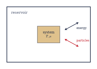
Fig. 448 The grand canonical ensemble. A small system (amber) sits in a large reservoir (the surroundings) with which it exchanges both energy (the wavy arrow) and particles (the straight arrow), at fixed temperature \(T\) and chemical potential \(\mu\). The microcanonical ensemble fixes \(E\) and \(N\); the canonical ensemble (§5.8) frees \(E\) at fixed \(T\); the grand canonical ensemble frees \(N\) as well at fixed \(\mu\). Its probabilities carry one Boltzmann factor for the energy and one for the number, \(P_s\propto e^{-\beta(E_s-\mu N_s)}\), and its master potential is the grand potential \(\Phi=-kT\ln\Xi\) of §5.7.#
Exercise 2 — The open ideal gas: \(\Xi=e^{zZ_1}\) and Poisson particle number (worked)#
The grand canonical ensemble proves its worth immediately for the ideal gas, and it hands us back an old
friend. Because the gas is non-interacting, its \(N\)-particle partition function is \(Z_N=Z_1^N/N!\)
(the factorization of §5.8, with the Gibbs \(1/N!\) of §5.6), so the grand sum is just the exponential
series, \(\Xi=\sum_N(zZ_1)^N/N!=e^{zZ_1}\) Eq. 431. Reading off the term for each \(N\), the
probability that the open system contains exactly \(N\) particles is \(P(N)=(zZ_1)^N e^{-zZ_1}/N!\) — a
Poisson distribution, precisely the law we built in §5.2 for rare independent events, now
arrived at as the equilibrium particle statistics of an open ideal gas (Fig. 449).
Its mean is \(\langle N\rangle=zZ_1\), and its defining signature is that the variance equals the
mean, \(\operatorname{Var}(N)=\langle N\rangle\), so the relative fluctuation is \(\sigma_N/\langle
N\rangle=1/\sqrt{\langle N\rangle}\) — already the \(1/\sqrt N\) that will prove the ensembles
equivalent. The factorial overflows for any real gas, so the pmf has to be evaluated in log
space: \(\ln P=N\ln\lambda-\lambda-\ln\Gamma(N+1)\) with scipy.special.gammaln, exponentiated
at the end — the §5.3/§0.1 lesson applied to the pmf
§5.2 built with an honest factorial. The moments are sums over all \(N\), so a truncated
range would bias them downward; carrying \(N\) out to \(\lambda+12\sqrt\lambda\) — twelve standard
deviations — leaves a discarded tail far below machine precision. The specimen here is
\(Z_1=10\) at fugacity \(z=2\), so \(\langle N\rangle=zZ_1=20\).
Write
poisson_pmf_logspace(N, lam), the pmf \(\lambda^Ne^{-\lambda}/N!\) evaluated through the logarithm above, accepting an array of particle numbersN. Write this one yourself — the implementation is the lesson.Write
grand_canonical_ideal_gas(z, Z1), which sets \(\lambda=zZ_1\), lays the pmf on the truncated range, and returns{"lam", "mean_N", "var_N"}with \(\langle N\rangle=\sum NP(N)\) and \(\operatorname{Var}(N)=\sum(N-\langle N\rangle)^2P(N)\).Run it on the specimen and confirm \(\langle N\rangle=\operatorname{Var}(N)=zZ_1\) and \(\sigma_N/\langle N\rangle=1/\sqrt{\langle N\rangle}\).
open ideal gas, zZ₁ = 20.0:
  ⟨N⟩ = 20.0000,  Var(N) = 20.0000   (Poisson: ⟨N⟩ = Var(N))
  σ_N/⟨N⟩ = 0.2236   vs   1/√⟨N⟩ = 0.2236
→ the open ideal gas's particle number is the Poisson distribution of §5.2
Validation 2#
✓  the open ideal gas has Poisson particle number, ⟨N⟩ = Var(N) = zZ₁   [max|Δ| = 7.10543e-14 (rtol=0.001, atol=1e-09)]
✓  the relative number fluctuation is σ_N/⟨N⟩ = 1/√⟨N⟩   [got 0.223607 vs expected 0.223607 (rtol=0.001, atol=1e-09)]
True
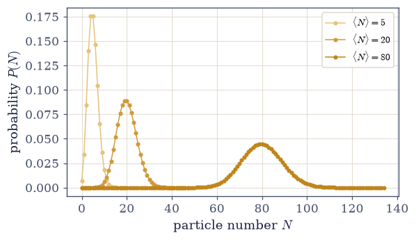
Fig. 449 The open ideal gas has Poisson particle number. The probability \(P(N)\) that an open subvolume holds \(N\) particles, for three values of the mean \(\langle N\rangle=zZ_1\) (computed in log space via gammaln). Each is a Poisson distribution — the §5.2 law for rare independent events — with \(\operatorname{Var}(N)=\langle N\rangle\). As \(\langle N\rangle\) grows the distribution broadens absolutely but narrows relatively: the relative width \(\sigma_N/\langle N\rangle=1/\sqrt{\langle N\rangle}\) shrinks, so a macroscopic open system has an essentially sharp particle number — the first sign that the grand canonical and canonical ensembles agree.#
Exercise 3 — Number fluctuations and the compressibility (worked)#
Now the first new fluctuation–response relation, and the central one of this notebook. We saw the variance of \(N\) equals its mean for the ideal gas; the deeper statement is why a variance should be a response at all. Differentiating \(\ln\Xi\) once gives the mean number, \(\langle N\rangle= \tfrac1\beta\partial\ln\Xi/\partial\mu\); differentiating again gives the variance, so \(\operatorname{Var}(N)=kT(\partial\langle N\rangle/\partial\mu)_{T,V}\) Eq. 432. The right-hand side is a response function: how much the particle number changes when we nudge the chemical potential. A little thermodynamics turns it into the isothermal compressibility, \(\operatorname{Var}(N)=\langle N\rangle^2kT\kappa_T/V\) with \(\kappa_T=-\tfrac1V(\partial V/\partial P)_T\). The physical reading is immediate: a nearly incompressible system (small \(\kappa_T\)) has small number fluctuations — squeeze it and nothing gives — while a system whose compressibility diverges has macroscopic number fluctuations. For the ideal gas both forms collapse to \(\operatorname{Var}(N)=\langle N\rangle\), the Poisson result, which is the check.
The second form has to be handled carefully, because it is easy to check it vacuously. Assigning \(\kappa_T=V/(\langle N\rangle kT)\) makes \(\langle N\rangle^2kT\kappa_T/V\) collapse to \(\langle N\rangle\) by pure algebra, testing nothing. So the compressibility must come from an independent route: its definition \(\kappa_T=-\tfrac1V(\partial V/\partial P)_T\), applied to the ideal-gas isotherm \(V(P)=NkT/P\) of §5.6 and differentiated numerically about the working point. Take \(V=Z_1\) in these units, at the \(\beta=1\), \(\mu=0.5\), \(Z_1=10\) of Exercises 1 and 2.
Compute \(kT(\partial\langle N\rangle/\partial\mu)\) by differentiating \(\langle N\rangle(\mu)=e^{\beta\mu}Z_1\) with
numpy.gradientover a narrow \(\mu\) grid, and confirm it equals \(\operatorname{Var}(N)=\langle N\rangle\).Measure \(\kappa_T\) from the isotherm as above, and confirm the compressibility form \(\langle N\rangle^2kT\kappa_T/V\) returns the same number.
ideal gas at μ=0.5: ⟨N⟩ = 16.4872
  kT(∂⟨N⟩/∂μ)      = 16.4876
  ⟨N⟩²kTκ_T/V       = 16.4873
  Var(N) = ⟨N⟩      = 16.4872   (all equal — fluctuation = compressibility response)
Validation 3#
✓  the particle-number variance equals kT(∂⟨N⟩/∂μ) — the compressibility (fluctuation = response)   [got 16.4876 vs expected 16.4872 (rtol=0.001, atol=1e-09)]
✓  the same variance equals ⟨N⟩²kTκ_T/V, with κ_T measured from the isotherm   [got 16.4873 vs expected 16.4872 (rtol=0.001, atol=1e-09)]
True
Exercise 4 — The fluctuation–response principle, collected (worked)#
We pause to gather what is becoming a pattern into a single principle, because it is one of the most useful ideas in the subject and deserves to be seen whole. Three times now a variance has turned out to equal a response function (Fig. 450). The canonical energy fluctuation was the heat capacity, \(\operatorname{Var}(E)=kT^2C_V\) (§5.8). The grand-canonical number fluctuation is the compressibility, \(\operatorname{Var}(N)=kT(\partial\langle N\rangle/\partial\mu) \propto\kappa_T\) (just now). And the magnetization fluctuation is the susceptibility, \(\operatorname{Var}(M)=kT\chi\) — the relation that will diverge at the Ising critical point of §5.10. These are one theorem, the static fluctuation–dissipation theorem: a susceptibility — the derivative of an extensive variable with respect to its conjugate intensive field — equals the variance of that variable, up to a factor of \(kT\) (\(kT^2\) for the energy–heat-capacity pair). The reason is always the same, that both the response and the variance are second derivatives of the same free energy. The practical power is enormous: to measure a response function in a simulation one need not apply a field and measure the change — one simply lets the system sit at equilibrium and watches it fluctuate. This is exactly how \(C_V\) came out of the Metropolis energy fluctuations in §5.8, and how \(\kappa_T\) and \(\chi\) are obtained in practice.
The instance to check numerically is the energy–heat-capacity one, on the two-state spin of §5.8 at \(T=1\): there \(\ln Z=\ln(2\cosh\beta\varepsilon)\), and the heat capacity has the closed form \(C_V=(\varepsilon/T)^2\operatorname{sech}^2\beta\varepsilon\). The variance must come from somewhere else, or the check is an identity — so take it as the second \(\beta\)-derivative of \(\ln Z\), \(\operatorname{Var}(E)=\partial^2\ln Z/\partial\beta^2\), by a central finite difference at step \(h=10^{-4}\), and let the closed form grade the measurement. It then stands beside the number–compressibility instance of Exercise 3: two members of the one family.
Measure \(\operatorname{Var}(E)\) as that central second difference of \(\ln Z\).
Confirm \(\operatorname{Var}(E)/kT^2=C_V\) against the closed form.
the fluctuation–response family (each variance is a response function):
  energy ↔ heat capacity:     Var(E)/kT² = 0.419974   vs   C_V = 0.419974
  number ↔ compressibility:   Var(N) = kT(∂⟨N⟩/∂μ)        (Exercise 3)
  magnetization ↔ susceptibility: Var(M) = kT χ           (→ diverges at the Ising T_c, §5.10)
Validation 4#
✓ Var(E) measured as ∂²lnZ/∂β² equals kT²C_V — a fluctuation–response relation [got 0.419974 vs expected 0.419974 (rtol=1e-06, atol=1e-09)]
True
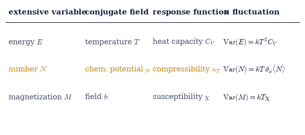
Fig. 450 The fluctuation–response family: one principle, three instances. For each conjugate pair, the variance of the extensive variable equals the response function — the derivative of that variable with respect to its conjugate intensive field — up to \(kT\) (\(kT^2\) for the energy–heat-capacity pair). This is the static fluctuation–dissipation theorem: response is fluctuation, because both are second derivatives of the same free energy. Its practical force is that a simulation measures a response function by watching the system jitter at equilibrium, with no field applied — exactly how the heat capacity came out of the Metropolis run in §5.8.#
Exercise 5 — The canonical energy distribution narrows onto the microcanonical value (worked)#
We turn to the equivalence of ensembles, and the mechanism is the sharpness of fluctuations. A canonical system does not have a definite energy — it trades energy with its bath — so strictly it is described by a distribution of energies, \(P(E)\propto\Omega(E)e^{-\beta E}\): the number of microstates at energy \(E\) (rising fast) times the Boltzmann suppression (falling fast). The product is sharply peaked, and the peak sits exactly where \(\partial\ln\Omega/\partial E=\beta\), i.e. where \(\partial S/\partial E=1/T\) — which is the microcanonical energy at temperature \(T\) Eq. 433. So the canonical ensemble’s most probable energy is the microcanonical energy; the only question is how tightly it is pinned there. The answer is the \(1/\sqrt N\) of §5.3: the relative width \(\sigma_E/\langle E\rangle\) shrinks as \(1/\sqrt N\) (Fig. 451), from of order one for a handful of spins to a part in a thousand by \(N=10^6\). As \(N\to\infty\) the canonical energy distribution becomes a spike at the microcanonical value — the two ensembles describe the same state.
The specimen is \(N\) two-state spins at \(\beta=1\), the system of §5.8. Each spin has
energy \(\pm\varepsilon\), so with \(n_\uparrow\) spins in the \(+\varepsilon\) state the total
energy is \(E=(2n_\uparrow-N)\varepsilon\) and the multiplicity is the binomial coefficient
\(\Omega=\binom{N}{n_\uparrow}\) — which at \(N=2000\) is a number no float can hold, so
\(P(E)\propto\Omega(E)e^{-\beta E}\) has to be assembled in log space: \(\ln\Omega\) from
scipy.special.gammaln as in §5.3, the largest log-weight subtracted before exponentiating,
and the result normalized to sum to one. The microcanonical energy per spin at this
temperature is \(-\tanh\beta\varepsilon\), and the relative width should fall from
\(\approx0.60\) at \(N=2\) to \(\approx0.019\) at \(N=2000\) — a factor of \(\sqrt{1000}\) for a
thousandfold \(N\).
Write
canonical_energy_distribution(N, beta, eps=1.0), returning(E, P)— the energy values and their probabilities — by the log-space construction above. Write this one yourself — the implementation is the lesson.Build it at \(\beta=1\) for \(N=2,20,200,2000\); confirm the mean energy per spin equals the microcanonical \(-\tanh\beta\varepsilon\), and that the relative width \(\sigma_E/|\langle E\rangle|\) falls as \(1/\sqrt N\).
Animate the distribution as \(N\) doubles from \(2\) to \(1024\), against the fixed microcanonical energy it must collapse onto — the narrowing is motion, which a still cannot show.
N=    2: ⟨E⟩/N = -0.7616 (micro -0.7616);  σ_E/|⟨E⟩| = 0.6017  (0.851/√N = 0.6017)
N=   20: ⟨E⟩/N = -0.7616 (micro -0.7616);  σ_E/|⟨E⟩| = 0.1903  (0.851/√N = 0.1903)
N=  200: ⟨E⟩/N = -0.7616 (micro -0.7616);  σ_E/|⟨E⟩| = 0.0602  (0.851/√N = 0.0602)
N= 2000: ⟨E⟩/N = -0.7616 (micro -0.7616);  σ_E/|⟨E⟩| = 0.0190  (0.851/√N = 0.0190)
Validation 5#
✓  the canonical energy distribution peaks at the microcanonical energy −tanh βε   [got -0.761594 vs expected -0.761594 (rtol=0.01, atol=1e-09)]
✓  the canonical energy fluctuation vanishes as 1/√N (the relative width scales as N^(−1/2))   [got 0.850918 vs expected 0.850918 (rtol=0.01, atol=1e-09)]
True
Fig. 451 The canonical energy distribution collapses onto the microcanonical value (animated). The distribution of energy per spin \(P(E/N)\) for \(N\) two-state spins at \(\beta=1\), as \(N\) grows. For a few spins it is broad; as \(N\) increases it narrows — relative width \(\propto1/\sqrt N\) — onto the microcanonical energy \(-\tanh\beta\varepsilon\) (dashed). At macroscopic \(N\) the canonical ensemble, though it nominally lets the energy fluctuate, pins it as tightly as the microcanonical ensemble that fixes it: the two are equivalent. This narrowing is the \(1/\sqrt N\) sharpening of §5.3, and it is the engine of the equivalence of ensembles.#
Exercise 6 — The grand-canonical particle number narrows onto the canonical value (worked)#
The same collapse happens on the particle-number side, and it completes the chain. The grand canonical ensemble lets \(N\) fluctuate, with the Poisson distribution of Exercise 2; but that distribution’s relative width is \(\sigma_N/\langle N\rangle=1/\sqrt{\langle N\rangle}\) Eq. 433, which vanishes as the system grows. So a macroscopic open system has, for all thermodynamic purposes, a fixed particle number equal to \(\langle N\rangle\) — the canonical value (Fig. 449 already showed the relative narrowing). Put the two collapses together: the canonical energy distribution pins onto the microcanonical energy (Exercise 5), and the grand-canonical number distribution pins onto the canonical number (here). The three ensembles, which differ only in what they let fluctuate, become indistinguishable once the fluctuations are negligible — which, by §5.3, they are at macroscopic \(N\).
The mean occupations to sweep are \(\langle N\rangle=5,50,500,5000\), obtained from the
grand_canonical_ideal_gas you wrote in Exercise 2 by setting \(z=1\) and \(Z_1=\langle N
\rangle\), so each decade should shrink the relative fluctuation by \(\sqrt{10}\).
Compute \(\sigma_N/\langle N\rangle\) at those four occupations and confirm each equals \(1/\sqrt{\langle N\rangle}\), so it \(\to0\) in the thermodynamic limit — the grand canonical ensemble effectively fixing \(N\) at the canonical value.
grand-canonical particle number, relative fluctuation σ_N/⟨N⟩:
  ⟨N⟩ =       5: σ_N/⟨N⟩ = 0.44721   vs   1/√⟨N⟩ = 0.44721
  ⟨N⟩ =      50: σ_N/⟨N⟩ = 0.14142   vs   1/√⟨N⟩ = 0.14142
  ⟨N⟩ =     500: σ_N/⟨N⟩ = 0.04472   vs   1/√⟨N⟩ = 0.04472
  ⟨N⟩ =    5000: σ_N/⟨N⟩ = 0.01414   vs   1/√⟨N⟩ = 0.01414
→ as ⟨N⟩ grows the open system's number is pinned at the canonical value (ensembles agree)
Validation 6#
✓ the grand-canonical number collapses onto the canonical value as σ_N/⟨N⟩ = 1/√⟨N⟩ [max|Δ| = 2.10387e-14 (rtol=0.001, atol=1e-09)]
True
Exercise 7 — One quantity, three ensembles, one answer (worked)#
Here is the payoff the whole notebook has been driving at. If the ensembles are equivalent, then a thermodynamic quantity computed in any of them must give the same number — and we can simply check it. We take the energy per particle of the ideal gas and compute it three ways Eq. 433: microcanonically, from \(1/T=\partial S/\partial E\), which gives \(E=\tfrac32NkT\) and so \(\tfrac32 kT\) per particle (the equipartition of §5.6); canonically, as \(-\partial\ln Z_1/\partial\beta= \tfrac32kT\); and grand-canonically, as \(\langle E\rangle/\langle N\rangle\), the Poisson-weighted energy over the Poisson-weighted number, again \(\tfrac32kT\). The three agree exactly. What distinguishes the ensembles is only their fluctuations — the canonical energy spread and the grand-canonical number spread — and those both vanish as \(1/\sqrt N\) (Fig. 452). So the freedom is real and practical: compute any quantity in whichever ensemble is most convenient (often the grand canonical, where the unconstrained sums factorize most easily), confident that the thermodynamic-limit answer is ensemble-independent.
The quantity is the ideal-gas energy per particle at \(T=1\), in the \(V=Z_1\) box of Exercise 3.
The single-particle partition function is \(Z_1=V(2\pi/\beta)^{3/2}\propto\beta^{-3/2}\), so
\(\ln Z_1=\ln V-\tfrac32\ln(\beta/2\pi)\), and both derivative routes are taken with
numpy.gradient over a narrow \(\beta\) grid. The grand-canonical route needs care for the same
reason Exercise 3’s did: writing \(\langle E\rangle=\tfrac32kT\sum NP(N)\) and dividing by
\(\langle N\rangle=\sum NP(N)\) cancels identically and tests nothing. Take it instead from the
grand potential — \(\ln\Xi=zZ_1\) gives \(\langle E\rangle=-z\,\partial Z_1/\partial\beta\) and
\(\langle N\rangle=zZ_1\), so the per-particle energy is \(-(\partial Z_1/\partial\beta)/Z_1\)
with the fugacity cancelling, and it is \(Z_1(\beta)\) itself, not its logarithm, that gets
differenced: a genuinely distinct numerical path to the same \(\tfrac32kT\).
Write down the microcanonical value, \(E=\tfrac32NkT\) and so \(\tfrac32kT\) per particle.
Compute the canonical value as \(-\partial\ln Z_1/\partial\beta\).
Compute the grand-canonical value as \(-(\partial Z_1/\partial\beta)/Z_1\), and confirm all three agree.
Plot the two distinguishing fluctuations — the canonical energy spread and the grand-canonical number spread — vanishing together as \(1/\sqrt N\).
ideal-gas energy per particle, computed three ways:
  microcanonical  = 1.50000
  canonical       = 1.50008
  grand canonical = 1.50034     (all = 3/2 kT = 1.5)
Validation 7#
✓ the three ensembles give the same per-particle energy in the thermodynamic limit [max|Δ| = 0.000341863 (rtol=0.001, atol=1e-09)]
True
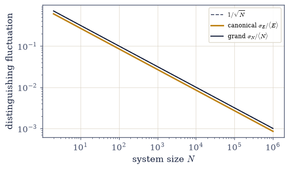
Fig. 452 What distinguishes the ensembles vanishes as \(1/\sqrt N\). The energy per particle is identical in all three ensembles (Validation 7); what differs is only their fluctuations. The canonical energy spread \(\sigma_E/\langle E\rangle\) (amber, for two-state spins) and the grand-canonical number spread \(\sigma_N/\langle N\rangle\) (dark, Poisson) both fall as \(1/\sqrt N\) (dashed). By macroscopic \(N\) they are negligible, so the microcanonical, canonical, and grand canonical ensembles are interchangeable — one chooses whichever is most convenient. The equivalence of ensembles is a direct consequence of the \(1/\sqrt N\) sharpening of §5.3.#
Exercise 8 — Measuring a response function from fluctuations (student)#
The fluctuation–response principle is not only an identity to admire; it is a working tool, and this exercise turns it into one. The claim of Exercise 4 was that a response function equals a fluctuation, so we ought to be able to measure a response — say the heat capacity — without ever changing the temperature and watching the energy respond. Instead we let the system sit at one temperature, sample its equilibrium energy with the Metropolis algorithm of §5.8, measure the variance of that energy, and divide by \(kT^2\). For \(N\) two-state spins at \(\beta=1\) this should return the exact per-spin heat capacity \((\varepsilon/T)^2\operatorname{sech}^2\beta\varepsilon\). It does, to sampling accuracy — which is precisely how heat capacities, compressibilities, and susceptibilities are extracted from Monte Carlo and molecular-dynamics runs in practice (and in MMM). Response from fluctuation, measured.
Take \(N=2000\) independent spins at \(\beta=1\), run \(5000\) sweeps with a seeded
numpy.random.default_rng(0), and discard the first \(1000\) as burn-in. Because the spins are
independent, one sweep is a single vectorized step: flipping spin \(\sigma\) costs
\(\Delta E=-2\sigma\varepsilon\), and the Metropolis rule \(\min(1,e^{-\beta\Delta E})\) accepts
wherever rng.random(N) < np.exp(-beta*dE) — no if, no loop over spins, the whole lattice
updated at once. The total energy of a configuration is \(\sum_i\sigma_i\varepsilon\), and the
exact answer to compare against is the closed form of Exercise 4,
\(C_V/N=(\varepsilon/T)^2\operatorname{sech}^2\beta\varepsilon\).
Write the sweep loop: propose the flip of every spin, accept by the vectorized Metropolis rule, and record the total energy after the burn-in. Write this one yourself — the implementation is the lesson.
Measure the energy variance of the recorded chain and recover the per-spin heat capacity \(C_V/N=\operatorname{Var}(E)/(NkT^2)\), comparing it with the exact value.
N=2000 two-state spins, β=1.0:
  C_V/N from fluctuations  Var(E)/(NkT²) = 0.4312
  C_V/N exact  (ε/T)²sech²βε             = 0.4200
→ a response function read straight off the equilibrium energy jitter
Validation 8#
✓ a response function (the heat capacity) can be measured from equilibrium energy fluctuations [got 0.43121 vs expected 0.419974 (rtol=0.08, atol=1e-09)]
True
Exercise 9 — Where the equivalence breaks: the critical point (worked)#
We end at the one place all of this machinery strains, because that is where the interesting physics begins. Everything in this notebook rested on fluctuations being small — vanishing as \(1/\sqrt N\) — which made the ensembles equivalent. But the fluctuation–response relations cut both ways: if a response function diverges, then so do the fluctuations Eq. 434. A diverging susceptibility, \(\chi\to\infty\), means a diverging magnetization variance, \(\operatorname{Var}(M)=kT\chi\to\infty\) — fluctuations that do not shrink as \(1/\sqrt N\) but instead grow to span the entire system (Fig. 453). At such a critical point the different ensembles can give different answers, and the clean equivalence we proved fails. This is not a defect of the theory; it is the theory pointing at where the physics is richest. A diverging susceptibility with system-spanning fluctuations is the fingerprint of a phase transition — and the Ising model of §5.10 is exactly this story: as the temperature approaches \(T_c\) the susceptibility blows up, fluctuations correlate across the whole magnet, and spontaneous order appears out of a model with no built-in preference. The whole ensemble apparatus has been building toward the place where it most dramatically breaks.
What follows is a stated model of critical behaviour, not a measurement: a susceptibility \(\chi=1/|T-T_c|\) that diverges at \(T_c=2.27\), the two-dimensional Ising critical temperature of Onsager, approached from above along \(T\in[T_c+0.04,\,T_c+2.5]\). The measured version is the capstone of §5.10, where this figure comes true. Across that approach the divergence should be unmistakable — both quantities growing by more than a factor of ten.
Build the model susceptibility on the approach grid.
Form \(\operatorname{Var}(M)=kT\chi\) from it and confirm that response and fluctuation diverge in lock-step — the signature of a critical point, where ensemble equivalence fails.
model critical point at T_c = 2.27:
  approaching T_c: χ rises 0.40 → 25.00, and Var(M)=kTχ rises 1.91 → 57.75
  growth over the approach: χ ×62, Var(M) ×30
→ a diverging response is a diverging fluctuation — the fluctuations span the system (§5.10)
Validation 9#
✓ in the model, response and fluctuation diverge together approaching T_c — where ensemble equivalence fails (the §5.10 preview)
True
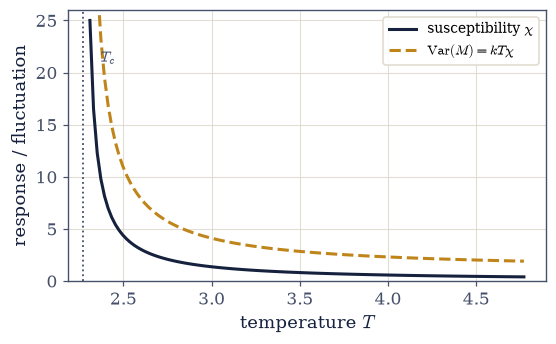
Fig. 453 Where ensemble equivalence breaks. A susceptibility that diverges at a critical temperature \(T_c\) (dark), \(\chi\propto1/|T-T_c|\), and the magnetization fluctuation \(\operatorname{Var}(M)=kT\chi\) that diverges with it (amber) by the fluctuation–response relation. Unlike the \(1/\sqrt N\) fluctuations that made the ensembles equivalent, these fluctuations grow without bound — they span the whole system. A diverging response is a diverging fluctuation, and that is the fingerprint of a phase transition: the Ising critical point of §5.10, where the susceptibility blows up and spontaneous order emerges.#
Exercise 10 — One theory, three ensembles, and the role of fluctuations (synthesis)#
Look back at the structure now complete. We built three ensembles — microcanonical, canonical, and grand canonical — distinguished only by what they hold fixed and what they let fluctuate: energy and number, then just number, then nothing. We proved them one, and the proof was fluctuations: the canonical energy distribution pins onto the microcanonical energy, the grand-canonical number pins onto the canonical number, each with a relative width that vanishes as \(1/\sqrt N\) (§5.3), so in the thermodynamic limit the three describe the same physics and one is free to choose the most convenient. Along the way the fluctuations turned out to be the response functions — the heat capacity, the compressibility, the susceptibility — the static fluctuation–dissipation theorem, which is how response is measured in practice. And the one place the fluctuations do not vanish, the critical point, is exactly where the next notebook goes.
There is no new computation to do: the architecture is the result. Three ensembles, proven equivalent by the smallness of fluctuations; fluctuations that are themselves the response functions; and a single exception — the critical point — where the fluctuations grow without bound. That exception is the doorway to §5.10: the Ising model, where a diverging susceptibility and system-spanning fluctuations produce a genuine phase transition and the spontaneous emergence of order.
Notebook summary#
This notebook completed the ensemble theory and made fluctuations its spine: the grand canonical ensemble, the fluctuation–response relations, and the equivalence of ensembles.
The grand canonical ensemble Eq. 430: a system open to energy and particle exchange at fixed \((T,\mu)\) has \(P_s=e^{-\beta(E_s-\mu N_s)}/\Xi\), with the grand potential \(\Phi=-kT\ln\Xi\) of §5.7 grounded statistically.
The open ideal gas Eq. 431: \(\Xi=e^{zZ_1}\) and the particle number is Poisson (the §5.2 payoff), \(\langle N\rangle=\operatorname{Var}(N)=zZ_1\), \(\sigma_N/\langle N\rangle= 1/\sqrt{\langle N\rangle}\), computed in log space via
gammaln.Fluctuation–response Eq. 432: \(\operatorname{Var}(E)=kT^2C_V\) (§5.8), \(\operatorname{Var}(N)=kT\partial_\mu\langle N\rangle\propto\kappa_T\) (here, both forms verified), \(\operatorname{Var}(M)=kT\chi\) — one theorem, response is fluctuation, and the way simulations measure response functions.
Equivalence of ensembles Eq. 433: the canonical energy distribution peaks at the microcanonical energy with width \(\propto1/\sqrt N\) (\(0.60\to0.019\) for \(N=2\to2000\)), and the grand-canonical Poisson number collapses as \(1/\sqrt{\langle N\rangle}\); one quantity computed three ways agrees (\(\tfrac32kT\) per particle).
The critical point Eq. 434: a diverging response is a diverging fluctuation that does not vanish as \(1/\sqrt N\) — where equivalence breaks and the physics gets interesting.
Three ensembles, proven one by the smallness of fluctuations; fluctuations that are the response functions; and one exception — the critical point — that is the doorway to the volume’s capstone.
Outlook#
The Ising model (§5.10). The critical point where the susceptibility diverges, fluctuations span the system, ensemble equivalence strains, and spontaneous order emerges — the volume’s capstone, computed with the Metropolis algorithm of §5.8.
The fluctuation–dissipation theorem, in full. Its dynamical form relates equilibrium fluctuations to the response to time-dependent perturbations — a pointer beyond this volume.
Open and reacting systems. The grand canonical ensemble is the natural language for adsorption, chemical equilibrium, and phase coexistence — the chemical potential of §5.6 in action.
Quantum statistics (Volume VII). The same \(\Xi\) with quantum \(Z_N\) gives Fermi–Dirac and Bose–Einstein statistics in the occupation-number formalism — once Volume VI builds the quantum mechanics.
Cross-reference §5.2 (Poisson), §5.3 (\(1/\sqrt N\), large-\(N\)), §5.7 (\(\Phi\), response functions), §5.8 (energy fluctuations, \(\operatorname{Var}(E)=kT^2C_V\)).