


0.9 Symbolic Computation with SymPy#
Notebook overview#
Volume 0 opened with an uncomfortable fact: the computer does not do real arithmetic. §0.1 showed \(0.1 + 0.2 \ne 0.3\) and traced every later wobble back to that finite grid. This closing notebook answers the question §0.1 quietly raised. If floating point is so treacherous, can we just compute exactly? Sometimes, yes. A computer algebra system (CAS) manipulates mathematical expressions the way we do by hand, with symbols and exact rationals rather than rounded decimals, and SymPy is that escape hatch in Python.
We will see SymPy do the things a CAS does well: differentiate by the chain and product rules mechanically, integrate in closed form when one exists, expand Taylor series, solve equations and small linear-algebra problems exactly. We will also see, just as honestly, where it stops. Most integrals and most equations have no closed form, which is exactly why Volume 0 spent so long on numerical root-finders (§0.2) and quadrature (§0.3): they answer the questions symbolic methods cannot. The two approaches are partners, each covering the other’s blind spot, and the working physicist keeps both hands.
The hinge between them is lambdify: derive an expression symbolically, then compile it to a fast numerical function for arrays. That single step is the workflow of §2.1, where SymPy derives an equation of motion from a Lagrangian and hands it to an ODE solver. The pendulum derivation in Exercise 7 is that whole pipeline in miniature, and it is where this volume’s tools and Volume II’s physics first meet.
There are no animations here. Symbolic manipulation is static by nature, and a printed expression or a single plotted trajectory says everything a moving picture would.
How to read the checks. Each exercise ends with a
validatecall against an independent fact: a symbolic difference that simplifies to zero, a known exact value, a lambdified function matching a direct evaluation. A ✓ is strong evidence; a ✗ is a prompt to locate the discrepancy, not a verdict. The habit matters even here: a CAS can apply an identity under assumptions one did not intend, so symbolic results deserve a check too.
Theory in brief#
Symbolic versus numeric#
Numerical computation manipulates floating-point approximations: every quantity is a 64-bit number on the grid of §0.1, and every operation rounds. Symbolic computation manipulates exact expressions: the symbol \(x\), the rational \(\tfrac{1}{10}\), the number \(\sqrt{2}\) are held exactly, never as decimals. So \(\tfrac{1}{10} + \tfrac{2}{10}\) is exactly \(\tfrac{3}{10}\) and \((\sqrt 2)^2\) is exactly \(2\), with no rounding anywhere. This is the clean escape from the error analysis of §0.1, and it has its own price.
What a CAS does well, and what it cannot#
A CAS excels at the mechanical parts of calculus and algebra: exact differentiation (the rules applied without slips), symbolic integration where a closed form exists, Taylor series, exact solving of equations and systems, exact linear algebra, and simplification. What it cannot do is conjure closed forms that do not exist. Most integrals have no elementary antiderivative and most equations have no formula for their roots, and there a CAS honestly returns a special function or nothing at all. That is precisely the gap the numerical methods of §0.2 and §0.3 were built to fill. Symbolic results can also suffer expression swell, growing huge and slow, which is a second reason to drop to numerics once a closed form stops helping.
The bridge: lambdify#
The two worlds meet through sympy.lambdify, which compiles a symbolic expression
into a fast NumPy function. The pattern is: derive symbolically for correctness,
then lambdify and evaluate numerically for speed. This is the exact workflow of
§2.1, where a symbolic
equation of motion becomes the right-hand side of an ODE solve.
Trust, but verify#
One caveat carries over from the rest of the course. A CAS applies identities under assumptions about domains and branch cuts, and those assumptions may not be the ones intended. A symbolic answer is therefore still a claim, to be checked against a known case or a numerical evaluation. The validation habit does not lapse just because the arithmetic is exact.
Setup#
Data and instruments only: the libraries, the one core symbol \(x\) that runs through the notebook, and SymPy’s Unicode pretty-printer. There is no method waiting here to be certified — the computer algebra is SymPy’s, and every derivation this notebook teaches (the limit-definition check, the Euler–Lagrange pipeline, the lambdify bridge) is carried out in its exercise.
The Setup below holds this notebook’s data and instruments — nothing you are asked to build. It is collapsed so the building stays yours; expand it whenever you want the details.
Exercise 1 — Exact arithmetic: the answer to 0.1#
§0.1 opened with \(0.1 + 0.2 \ne 0.3\), the headline symptom of finite-precision arithmetic. The first thing to see about a CAS is that this symptom simply does not appear: with exact rationals, the sum is the rational we expect, and surds square back to integers exactly.
Show that
sympy.Rational(1, 10) + sympy.Rational(2, 10)equals exactly \(\tfrac{3}{10}\), and contrast the float result \(0.30000000000000004\).Show that \((\sqrt 2)^2 = 2\) exactly (
sympy.sqrt).
symbolic:  1/10 + 2/10 = 3/10   (exactly three-tenths)
float   :  0.1 + 0.2   = 0.30000000000000004   (not 0.3)
symbolic:  (√2)² = 2   (exactly the integer 2)
Validation 1#
✓  symbolic arithmetic is exact: 1/10 + 2/10 is exactly 3/10   [got 3/10]
✓  a surd squares back to the exact integer: (√2)² = 2   [got 2]
True
Exercise 2 — Symbolic differentiation#
Differentiation is the most mechanical operation in calculus: the chain and product rules applied without error. A CAS does it perfectly, and we can confirm the result against the definition of the derivative, taken as a symbolic limit, so that nothing is assumed.
For the explicit function \(f(x) = \sin(x)\,e^{-x^2}\), compute \(f'(x)\) with
sympy.diff.Verify it equals the limit-definition derivative \(\lim_{h\to0}\big(f(x+h) - f(x)\big)/h\), taken symbolically with
sympy.limit— so nothing about differentiation is assumed.
f(x) = exp(-x**2)*sin(x)
f'(x) = (-2*x*sin(x) + cos(x))*exp(-x**2)
limit definition = (-2*x*sin(x) + cos(x))*exp(-x**2)
Validation 2#
✓ symbolic differentiation matches the limit definition of the derivative [difference simplifies to 0]
True
Exercise 3 — Symbolic integration, and its honest limit#
Integration is where a CAS first shows its edges. Some integrands have a clean antiderivative and SymPy returns it; some have a finite definite value expressible exactly; and many have no elementary antiderivative at all, where the best a CAS can do is name a special function. That last case is the callback to §0.3: it is exactly when one reaches for numerical quadrature.
For the explicit integrand \(x^2 e^{-x}\), compute the indefinite integral with
sympy.integrate(it is \((-x^2 - 2x - 2)e^{-x}\)).Compute the definite integral \(\int_0^\infty x^2 e^{-x}\,dx\) (it is \(2\), a value of the Gamma function).
Then try \(e^{-x^2}\), whose antiderivative is not elementary, and watch SymPy return the error function \(\operatorname{erf}\) — the honest signal to reach for the quadrature of §0.3.
∫ x²e^{−x} dx       = (-x**2 - 2*x - 2)*exp(-x)
∫₀^∞ x²e^{−x} dx    = 2
∫ e^{−x²} dx = sqrt(pi)*erf(x)/2 (no elementary form: erf appears)
Validation 3#
✓  ∫₀^∞ x²e^{−x} dx = 2 exactly (a Gamma-function value)   [got 2]
✓  e^{−x²} has no elementary antiderivative: SymPy returns erf (use quadrature, cf. §0.3)   [antiderivative = sqrt(pi)*erf(x)/2]
True
Exercise 4 — Taylor series#
Series expansions run through all of physics, from the small-angle pendulum to perturbation theory, and a CAS produces them on demand. The truncation that makes a series a finite approximation is the same one that set the step-size trade-offs of §0.1 and §0.3: keep more terms for more accuracy, at more cost.
Compute the Taylor series of \(\cos x\) about \(0\) to order \(10\) with
sympy.seriesand read off the coefficients (removeO, thencoeff).Confirm they are exactly \((-1)^n/(2n)!\) for the \(x^{2n}\) terms (the odd powers vanish).
cos(x) = 1 - x**2/2 + x**4/24 - x**6/720 + x**8/40320 - x**10/3628800 + O(x**11)
coefficients of x^(2n): [1, -1/2, 1/24, -1/720, 1/40320, -1/3628800]
(−1)ⁿ/(2n)!           : [1, -1/2, 1/24, -1/720, 1/40320, -1/3628800]
Validation 4#
✓ the cos Taylor coefficients are exactly (−1)ⁿ/(2n)! [[1, -1/2, 1/24, -1/720, 1/40320, -1/3628800] == [1, -1/2, 1/24, -1/720, 1/40320, -1/3628800]]
True
Exercise 5 — Exact equation solving (callback to 0.2)#
Here is the honest complement to §0.2. A CAS can solve some equations exactly, returning a formula rather than a number. The quadratic is the classic case: SymPy derives the very formula that §0.2 then evaluated numerically. But closed-form solutions are the lucky exception. The transcendental equations of §0.2 (a quantum energy condition) have no formula at all, which is why numerical root-finders exist.
Solve the general quadratic \(ax^2 + bx + c = 0\) symbolically with
sympy.solveand confirm the roots match the closed-form quadratic formula.Solve the explicit linear system \(x + y = 3\), \(x - y = 1\) exactly.
quadratic roots:
   (-b - sqrt(-4*a*c + b**2))/(2*a)
   (-b + sqrt(-4*a*c + b**2))/(2*a)
solution of x+y=3, x−y=1: {x: 2, y: 1}
Validation 5#
✓  SymPy derives the exact quadratic formula for ax²+bx+c=0   [roots [(-b - sqrt(-4*a*c + b**2))/(2*a), (-b + sqrt(-4*a*c + b**2))/(2*a)]]
✓  SymPy solves the linear system x+y=3, x−y=1 exactly (x=2, y=1)   [got {x: 2, y: 1}]
True
Exercise 6 — The bridge: lambdify#
This is the step that makes symbolic computation
practical for physics. Having derived an expression exactly, we compile it with
sympy.lambdify into a NumPy function that runs on whole arrays at numerical
speed. Symbolic for correctness, numeric for speed: the same two-stage workflow
§2.1 uses to turn a
Lagrangian into an integrable equation of motion.
Take the symbolic derivative \(f'(x)\) from Exercise 2 and compile it with
sympy.lambdifyinto a NumPy function.Evaluate it on an array.
Compare against a direct numerical evaluation of the hand-computed derivative \(e^{-x^2}(\cos x - 2x\sin x)\).
max |lambdify − direct| = 1.11e-16
Validation 6#
✓ lambdify produces a numerical function matching the direct evaluation [max|Δ| = 1.11022e-16 (rtol=1e-10, atol=1e-09)]
True
Exercise 7 — Deriving an equation of motion (student exercise)#
Now the payoff, and it is yours to assemble. The Euler–Lagrange equation turns a single scalar, the Lagrangian \(\mathcal L\), into the equation of motion,
and a CAS can carry out the differentiations exactly. (The equation is the stationarity condition \(\delta S = 0\) of Hamilton’s action principle; §2.1 sets out the formalism and points to the full derivation.) For a pendulum of mass \(m\) and length \(\ell\) with angle \(\theta(t)\), the Lagrangian is \(\mathcal L = \tfrac12 m\ell^2\dot\theta^2 + mg\ell\cos\theta\). This is the full §2.1 pipeline in miniature: derive, lambdify, integrate.
Build \(\mathcal L\) symbolically (
sympy.Functionfor \(\theta(t)\)) and apply the Euler–Lagrange operation Eq. 62 withsympy.diff.Solve for \(\ddot\theta\) (
sympy.solve) and show it is \(-(g/\ell)\sin\theta\).Lambdify the acceleration, integrate one swing numerically with
scipy.integrate.solve_ivp, and confirm the energy is conserved (Fig. 54).
Because the check tests the derivation (\(\ddot\theta + (g/\ell)\sin\theta = 0\)), a ✗ means “re-examine the Lagrangian or the Euler–Lagrange step,” never a problem with the plot.
Euler–Lagrange: l*m*(g*sin(theta(t)) + l*Derivative(theta(t), (t, 2))) = 0
θ̈ = -g*sin(theta(t))/l
Validation 7#
✓ the symbolic Euler–Lagrange derivation gives θ̈ = −(g/ℓ) sin θ [θ̈ = -g*sin(theta(t))/l]
True
Part 3, the bridge to numerics: substitute concrete parameters, lambdify the acceleration, and integrate one swing. The energy \(E = \tfrac12 m\ell^2\dot\theta^2 - mg\ell\cos\theta\) should stay flat, a check on the whole pipeline (cf. the conservation tests of Volumes I–II).
max relative energy drift over the swing = 1.38e-11
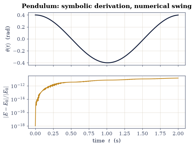
Fig. 54 One swing of the pendulum whose equation of motion \(\ddot\theta=-(g/\ell)\sin\theta\) was derived symbolically above, then lambdified and integrated with solve_ivp (\(g=9.81\), \(\ell=1\), \(\theta_0=0.4\) rad, released from rest). Top: the angle \(\theta(t)\). Bottom: the relative energy error \(|E(t)-E_0|/|E_0|\), flat at the solver-tolerance floor: the symbolic derivation and the numerical integration agree, exactly the §2.1 workflow.#
Validation 7b#
✓ the lambdified-and-integrated swing conserves energy (the pipeline is sound) [max relative energy drift = 1.38e-11]
True
Exercise 8 — Symbolic linear algebra, and where it stops#
Symbolic methods extend to linear algebra, and for small matrices they return exact eigenvalues, the closed-form complement to the numerical eigensolvers of §0.5. But the reach is short. Eigenvalues are roots of the characteristic polynomial, and by the Abel–Ruffini theorem there is no general formula for the roots of a polynomial of degree five or higher. So beyond small or special matrices, closed-form eigenvalues do not exist, which is exactly why the numerical algorithms of §0.5 are the everyday tool.
Compute the eigenvalues of the explicit matrix \(\begin{bmatrix} 2 & 1 \\ 1 & 2 \end{bmatrix}\) symbolically with
sympy.Matrix.eigenvals(they are exactly \(3\) and \(1\)).Note where the symbolic road ends: Abel–Ruffini forbids a general closed form at degree five and beyond, which is why the numerical algorithms of §0.5 are the everyday tool.
matrix M =
⎡2  1⎤
⎢    ⎥
⎣1  2⎦
symbolic eigenvalues (value: multiplicity): {3: 1, 1: 1}
Validation 8#
✓ the symbolic eigenvalues of [[2,1],[1,2]] are exactly 3 and 1 [got {3: 1, 1: 1}]
True
Notebook summary#
Exact arithmetic (the honest value of \(0.1\)), symbolic differentiation, symbolic integration and its genuine limits, Taylor series, and exact equation solving (callback to §0.2).
The
sympy.lambdifybridge from symbolic expressions to fast numeric functions, deriving an equation of motion symbolically, and symbolic linear algebra and where it stops being practical.
Outlook#
Assumptions and domains. Declaring
sp.symbols("x", positive=True)changes what simplifications are valid; a CAS can mislead when symbols are unconstrained, one more reason to verify.Code generation. Beyond
lambdify,sp.ccodeandsp.fcodeemit C and Fortran from symbolic expressions, which is how some simulation codes generate their force routines automatically.Expression swell. Symbolic results can grow huge and slow; knowing when to switch to numerics (or to a hybrid symbolic-numeric method) is part of the craft.
Forward links. Volume II leans on this workflow constantly (Lagrangians, Hamiltonians, Poisson brackets, normal-mode matrices), and the special functions met here reappear throughout the later volumes.
References#
Aaron Meurer and others. SymPy: symbolic computing in Python. PeerJ Computer Science, 3:e103, 2017. doi:10.7717/peerj-cs.103.
Wolfgang Nolting. Theoretical Physics 1: Classical Mechanics. Springer, 2016. Grundkurs Theoretische Physik 1.
Closing Volume 0#
This volume began by showing that the computer does not do real arithmetic, and it ends with the one tool that does. Everything in between (the root-finders, the quadrature, the linear algebra, the FFT, the ODE solvers) lives in the gap between exact and approximate, and the whole point of Volume 0 was to chart that gap honestly: to know what each method costs, where it breaks, and how to check that it worked. The working physicist keeps both hands. Reach for symbolic computation where a closed form exists and clarity demands it; reach for numerics everywhere else, which is most of the time! With the foundation laid, the physics can begin.