6.6 The Pauli Matrices, Incompatible Observables, and the Uncertainty Relation

Elementary Computational Physics

Volume VI — Quantum Mechanics Notebook 6.6

Why looking along x erases what we knew along z. The three spin components do not commute, and that single algebraic fact is the whole of the uncertainty principle: when two observables fail to commute, no state makes both sharp, and the product of their uncertainties is bounded below by their commutator. We build the Pauli algebra, derive the uncertainty relation from Cauchy–Schwarz, and find the states that meet it exactly.

Level · advanced   •   Est. · 150–185 min

Raymond Amador v1.4.0  ·  2026-07-31  ·  CC BY 4.0 (text) / MIT (code)

Notebook overview

The Stern–Gerlach experiment (§6.4) showed us, as a brute fact, that measuring spin along \(x\) destroys what we knew about spin along \(z\); the postulates (§6.5) gave us the variance \(\Delta A\) that measures how un-sharp an observable is in a state. This notebook supplies the missing piece — the algebra that explains why the destruction happens and how much it must — and it turns out to be one of the cleanest results in all of physics: the uncertainty principle is a three-line theorem about operators that do not commute.

The central new object is the commutator \([A,B]=AB-BA\). We met it in §6.2 as the test for whether two operators share an eigenbasis; here it becomes the protagonist. Two observables are compatible — can be simultaneously sharp in a common basis — exactly when they commute, and incompatible when they do not. The Pauli matrices are the canonical incompatible observables: the three spin components pairwise fail to commute, \([\sigma_x,\sigma_y]=2i\sigma_z\) and cyclically, so a state perfectly definite along one axis is maximally uncertain along the others. That is the sequential Stern–Gerlach experiment, now as algebra rather than anecdote.

The heart of the notebook is the derivation of the Robertson uncertainty relation \(\Delta A\, \Delta B\ge\tfrac12|\langle[A,B]\rangle|\). We do not assert it — we derive it, gently and in full, from the Cauchy–Schwarz inequality of §6.1, the very inequality that bounded probability amplitudes there. The lesson is worth stating plainly and is easy to get wrong: the uncertainty principle is not a statement about clumsy instruments disturbing delicate systems. It is a theorem about non-commuting Hermitian operators, true of every state whether or not anyone is looking, and it is saturated — met with equality — by special minimum-uncertainty states.

As in every Volume VI notebook, each exercise opens with a crystal-clear statement and enumerated parts, each naming the exact operation — explicit Pauli-matrix construction, commutator and anticommutator via the matrix-multiply @, numpy.vdot for the moments \(\langle A\rangle\) and \(\langle A^2\rangle\), and numpy.linalg.eigh where spectra are needed.

How to read the checks. Each exercise closes with a validate call: the full Pauli algebra (commutators, anticommutators, the product identity); the maximal uncertainty of \(\sigma_x\) in a \(\sigma_z\)-eigenstate; the Robertson inequality holding for random observables and states; its saturation by \(|{+}z\rangle\); and the simultaneous definiteness of commuting observables. A ✓ is strong evidence; a ✗ is a prompt to locate the discrepancy.

Conventions and scope. We work with \(\hbar=1\), so the spin operators are \(S=\tfrac12\boldsymbol \sigma\) with eigenvalues \(\pm\tfrac12\) (physically \(\pm\hbar/2\)); we restore \(\hbar\) in formulas where it clarifies. The qubit is the running example, with general Hermitian observables on \(\mathbb{C}^3\) for the general check. The position–momentum relation \(\Delta x\,\Delta p\ge\hbar/2\) from \([x,p]=i\hbar\) is §6.9; the angular-momentum algebra \([J_i,J_j]=i\hbar\varepsilon_{ijk}J_k\) is §6.14; complete sets of commuting observables catalogue the hydrogen atom in §6.17. See Sakurai & Napolitano (§1.4); Robertson (1929); Schrödinger (1930); and Notebooks §6.1 (Cauchy–Schwarz), §6.2 (commutators), §6.4 (the experiment), §6.5 (variance).

Theory in brief

The Pauli matrices and spin operators

The three Pauli matrices are the Hermitian observables of the qubit; the spin operators are \(S=\tfrac{\hbar}{2}\boldsymbol\sigma\),

(521)\[\begin{split}\sigma_x=\begin{pmatrix}0&1\\1&0\end{pmatrix},\ \sigma_y=\begin{pmatrix}0&-i\\i&0\end{pmatrix},\ \sigma_z=\begin{pmatrix}1&0\\0&-1\end{pmatrix},\qquad \sigma_i=\sigma_i^{\dagger},\ \sigma_i^2=I,\ \text{eigenvalues }\pm1 .\end{split}\]

They are exactly the observables a Stern–Gerlach magnet oriented along \(x\), \(y\), \(z\) measures (§6.4).

The algebra: commutators and the product identity

The commutator \([A,B]=AB-BA\) measures the failure to commute. The Pauli matrices satisfy

(522)\[[\sigma_x,\sigma_y]=2i\sigma_z\ (\text{cyclic}),\quad \{\sigma_i,\sigma_j\}=0\ (i\ne j),\quad \sigma_i\sigma_j=\delta_{ij}I+i\varepsilon_{ijk}\sigma_k ,\]

equivalently \([S_x,S_y]=i\hbar S_z\) — the angular-momentum algebra (generalized in §6.14). The commutator is zero for compatible observables and non-zero for incompatible ones.

Compatible versus incompatible observables

Two observables are compatible if \([A,B]=0\) — then (§6.2) they share an eigenbasis and can be simultaneously definite — and incompatible if \([A,B]\ne0\), when no common eigenbasis exists,

(523)\[[A,B]=0\ \Longleftrightarrow\ \text{simultaneously diagonalizable}\ \Longleftrightarrow\ \text{can be jointly sharp in a common basis} .\]

Concretely: in \(|{+}z\rangle\), where \(\sigma_z\) is perfectly definite, \(\langle\sigma_x\rangle=0\) and \((\Delta\sigma_x)^2=1\) — maximal uncertainty. This is the algebra of the sequential experiment.

The Robertson uncertainty relation — derived

For any two observables and any state,

(524)\[\Delta A\,\Delta B\ \ge\ \tfrac12\,\big|\langle[A,B]\rangle\big|,\qquad \Delta A=\sqrt{\langle A^2\rangle-\langle A\rangle^2} .\]

Derivation (Exercise 3). With the shifted operators \(\delta A=A-\langle A\rangle\), \(\delta B=B- \langle B\rangle\), the variance is \((\Delta A)^2=\langle\delta A^2\rangle\). Apply Cauchy–Schwarz (§6.1) to \(|\delta A\,\psi\rangle\) and \(|\delta B\,\psi\rangle\): \(\langle\delta A^2\rangle\langle\delta B^2\rangle\ge|\langle\delta A\,\delta B\rangle|^2\). Split \(\delta A\,\delta B=\tfrac12\{\delta A,\delta B\}+\tfrac12[A,B]\) into its Hermitian (anticommutator, real expectation) and anti-Hermitian (commutator, imaginary expectation) parts; dropping the anticommutator term keeps \(|\langle\delta A\, \delta B\rangle|^2\ge\big(\tfrac12|\langle[A,B]\rangle|\big)^2\), and the square root is the relation. It is Cauchy–Schwarz plus non-commutation — a theorem about operators, not instruments. (Keeping the anticommutator term gives the stronger Schrödinger relation; a pointer, not developed.)

Minimum-uncertainty states and complete sets

The inequality is saturated by special states,

(525)\[\text{for }(S_x,S_y):\quad |{+}z\rangle\ \text{gives}\ \Delta S_x\,\Delta S_y=\tfrac14=\tfrac12|\langle S_z\rangle| ,\]

the most “classical” allowed states (the Gaussian wave packet is their position–momentum analogue, §6.9). And commuting observables can be measured together and labelled by joint eigenvalues; a maximal commuting set — a complete set of commuting observables — labels states uniquely,

(526)\[\{A,B,\dots\}\ \text{mutually commuting and maximal}\ \Longrightarrow\ \text{joint eigenvalues label states uniquely} ,\]

which is how quantum states are catalogued (the hydrogen atom’s \(n,\ell,m,m_s\), §6.17).

Setup

Data and instruments only: the series palette, the three Pauli matrices Eq. 521 and the spin operators \(S=\tfrac12\boldsymbol\sigma\) they define, the commutator of §6.2 with its anticommutator companion, and the moment machinery of §6.5 — the expectation \(\langle A\rangle\) and the uncertainty \(\Delta A\) — restated here as tools. The new object this notebook is named for, the Robertson bound \(\tfrac12|\langle[A,B]\rangle|\), is deliberately absent: you write it in Exercise 3.

The Setup below holds this notebook’s data and instruments — nothing you are asked to build. It is collapsed so the building stays yours; expand it whenever you want the details.

Show code cell source

Hide code cell source

import matplotlib.pyplot as plt
import numpy as np

from ecp import draw, validate

ACCENT, INK, SOFT = draw.ACCENT, draw.INK, draw.SOFT  # data: the series palette

# Conventions: ℏ=1, so the spin operators are S = ½σ with eigenvalues ±½. Observables are
# Hermitian matrices; moments use numpy.vdot (conjugate-first, §6.1); commutators/anticommutators use the
# matrix-multiply @. The qubit is the running example; general checks use Hermitian matrices on ℂ³.

# data: the Pauli matrices (the SX/SY/SZ of §6.2), the canonical incompatible observables
SIGMA_X = np.array([[0, 1], [1, 0]], dtype=complex)
SIGMA_Y = np.array([[0, -1j], [1j, 0]], dtype=complex)
SIGMA_Z = np.array([[1, 0], [0, -1]], dtype=complex)
ID2 = np.eye(2, dtype=complex)
# data: the spin operators S = ½σ (ℏ = 1)
S_X, S_Y, S_Z = SIGMA_X / 2, SIGMA_Y / 2, SIGMA_Z / 2


# instrument: the AB−BA difference, met in §6.2 as the test for a shared eigenbasis — this
# notebook's lesson is what a non-zero commutator *implies* (incompatibility, and a floor
# under the uncertainty product), not the two-term difference that forms it.
def commutator(A, B):
    """The commutator $[A,B]=AB-BA$ {eq}`eq-pauli-algebra`.

    Computed with the matrix-multiply operator ``@``. It vanishes for compatible observables and is
    non-zero for incompatible ones; for Hermitian $A,B$ it is anti-Hermitian, so $\\langle[A,B]\\rangle$
    is purely imaginary — the fact that makes the uncertainty bound real.
    """
    return A @ B - B @ A


# instrument: the AB+BA companion to the commutator — plumbing for the algebra checks and
# for the Hermitian/anti-Hermitian split of Exercise 3; the lesson is what its expectation
# contributes to the bound, not the two-term sum itself.
def anticommutator(A, B):
    """The anticommutator $\\{A,B\\}=AB+BA$ {eq}`eq-pauli-algebra`.

    Computed with ``@``. For Hermitian $A,B$ it is Hermitian, so $\\langle\\{A,B\\}\\rangle$ is real; it
    is the term dropped in the Robertson relation and kept in the stronger Schrödinger relation.
    """
    return A @ B + B @ A


# built from scratch in §6.5 (the expectation value derived from the Born rule);
# restated here as an instrument.
def expectation(A, psi):
    """The expectation value $\\langle A\\rangle=\\langle\\psi|A|\\psi\\rangle$ (§6.5), via ``numpy.vdot``.

    Real because $A$ is Hermitian (``numpy.vdot(psi, A @ psi).real``).
    """
    return np.vdot(psi, A @ psi).real


# built from scratch in §6.5 (the variance and its vanishing on definite values);
# restated here as its square root, an instrument: ΔA is the quantity this notebook
# bounds, not a quantity it teaches you to form.
def dispersion(A, psi):
    """The uncertainty $\\Delta A=\\sqrt{\\langle A^2\\rangle-\\langle A\\rangle^2}$ {eq}`eq-uncertainty` (§6.5).

    The square root of the variance — zero exactly when ``psi`` is an eigenstate of ``A`` (a definite
    value). A small negative variance from rounding is clipped to zero before the square root.
    """
    var = expectation(A @ A, psi) - expectation(A, psi) ** 2
    return np.sqrt(max(var, 0.0))

Exercise 1 — The Pauli algebra

The three Pauli matrices are more than three convenient Hermitian \(2\times2\) matrices: they close among themselves under multiplication into an algebra Eq. 521, Eq. 522 — the commutation relations \([\sigma_x,\sigma_y]=2i\sigma_z\) and its cyclic partners, the anticommutation \(\{\sigma_i,\sigma_j\}=0\) for \(i \ne j\), the squares \(\sigma_i^2=I\), and the single product identity \(\sigma_i\sigma_j=\delta_{ij}I+i\varepsilon_{ijk}\sigma_k\) that contains all three. That algebra is the entire content of spin-\(\tfrac12\), and every result in this notebook is a consequence of it.

1. Take the matrices SIGMA_X, SIGMA_Y, SIGMA_Z from the setup.

2. Compute the three commutators with the commutator helper and confirm with numpy.allclose that they equal 2j*SIGMA_Z, 2j*SIGMA_X, 2j*SIGMA_Y.

3. Confirm the anticommutators anticommutator(SIGMA_i, SIGMA_j) vanish for \(i\ne j\) and that each SIGMA_i @ SIGMA_i equals ID2.

4. Verify the product identity on a representative pair, e.g. SIGMA_X @ SIGMA_Y equals 1j*SIGMA_Z. Note that \(S=\tfrac12 \sigma\) turns the first relation into the angular-momentum algebra \([S_x,S_y]=iS_z\) (\(\hbar=1\)).

[σx,σy]=2iσz: True; [σy,σz]=2iσx: True; [σz,σx]=2iσy: True
{σi,σj}=0 (i≠j): True;  σ²=I: True
product identity σxσy=iσz (cyclic): True;  with S=½σ this is [Sx,Sy]=iSz (ℏ=1)

Validation 1

✓  the Pauli matrices satisfy the full algebra: [σx,σy]=2iσz (cyclic), {σi,σj}=0 for i≠j, σ²=I, and σiσj=δijI+iεijkσk

True

Exercise 2 — The commutator as the test for compatibility

The sequential Stern–Gerlach destruction of §6.4 is governed by the commutator. \(\sigma_z\) and \(\sigma_x\) are incompatible (\([\sigma_z,\sigma_x]\ne0\)), so a state perfectly definite along \(z\) is maximally uncertain along \(x\); a compatible pair, one with a vanishing commutator, can instead be jointly sharp Eq. 523. For an observable with eigenvalues \(\pm1\) the largest variance any state can produce is \(1\), so “maximal” below is meant literally.

1. Compute \([\sigma_z,\sigma_x]\) with the commutator helper and confirm it is non-zero — incompatible.

2. In the \(\sigma_z\)-eigenstate \(|{+}z\rangle=\)numpy.array([1,0]), compute \(\langle\sigma_x\rangle\) with the expectation helper and \((\Delta\sigma_x)^2\) with the dispersion helper squared.

3. Find \(\langle\sigma_x\rangle=0\) and \((\Delta\sigma_x)^2=1\) — the maximum possible for an observable with eigenvalues \(\pm1\) (no common eigenbasis).

4. Contrast with the compatible pair \((\sigma_z,\sigma_z^2)\): \([\sigma_z,\sigma_z^2]=0\), and both are perfectly definite in \(|{+}z \rangle\). The contrast between the two pairs is the sequential experiment, told algebraically.

[σz,σx] ≠ 0 (incompatible): True
in |+z⟩:  ⟨σx⟩ = 0.000,  (Δσx)² = 1.000   (maximal — eigenvalues ±1)
[σz,σz²] = 0 (compatible): True;  both definite in |+z⟩: True

Validation 2

✓  an incompatible observable is maximally uncertain in an eigenstate of its partner: σx has ⟨σx⟩=0 and (Δσx)²=1 in |+z⟩   [max|Δ| = 0 (rtol=1e-06, atol=1e-12)]
✓  the commutator is the test for compatibility: [σz,σx]≠0 (incompatible, cannot be jointly sharp) while [σz,σz²]=0 (compatible, both definite)

True

Exercise 3 — Deriving the uncertainty relation

The Robertson relation is not asserted in this course; it is derived, and the derivation is three lines of Hilbert-space geometry Eq. 524. With the shifted operators \(\delta A=A-\langle A\rangle I\) and \(\delta B=B-\langle B\rangle I\) the variance is \((\Delta A)^2=\langle\delta A^2\rangle\); Cauchy–Schwarz (§6.1), applied to \(|\delta A\, \psi\rangle\) and \(|\delta B\,\psi\rangle\), bounds \(\langle\delta A^2\rangle\langle\delta B^2\rangle\ge|\langle\delta A\,\delta B\rangle|^2\); and the product splits as \(\delta A\,\delta B= \tfrac12\{\delta A,\delta B\}+\tfrac12[A,B]\) into a Hermitian part with real expectation and an anti-Hermitian part with purely imaginary expectation, so their squares simply add. Dropping the non-negative anticommutator square is what turns that equality into the inequality. The whole argument used nothing but the inner product, so it is checked below on random Hermitian observables on \(\mathbb{C}^3\) and a random state: the uncertainty principle is Cauchy–Schwarz plus non-commutation, and nothing else.

1. Write robertson_rhs(A, B, psi), the Robertson lower bound \(\tfrac12|\langle[A,B]\rangle|\) Eq. 524: half the magnitude of the commutator’s expectation value, 0.5 * numpy.abs(numpy.vdot(psi, commutator(A, B) @ psi)). It is the floor the rest of this exercise derives, and the object the notebook is named for.

2. Build Hermitian \(A,B\) on \(\mathbb{C}^3\) and a unit state, and form the shifted operators \(\delta A\) and \(\delta B\).

3. Verify the Cauchy–Schwarz step, \(\langle\delta A^2\rangle\langle\delta B^2\rangle\ge |\langle\delta A\, \delta B\rangle|^2\) (numpy.vdot for each inner product).

4. Confirm \(\langle\{\delta A,\delta B\}\rangle\) is real and \(\langle[A,B]\rangle\) purely imaginary, so \(|\langle\delta A\,\delta B\rangle|^2=\big(\tfrac12 \langle\{\delta A,\delta B\}\rangle\big)^2+\big(\tfrac12|\langle[A,B]\rangle|\big)^2\).

5. Confirm what survives when the anticommutator square is dropped: \(\Delta A\,\Delta B\ge\tfrac12|\langle[A,B]\rangle|\), your robertson_rhs against the product of two dispersion values.

(3) Cauchy–Schwarz ⟨δA²⟩⟨δB²⟩ = 49.2950 ≥ |⟨δAδB⟩|² = 20.1564: True
(4) ⟨{δA,δB}⟩ real (Im=-4.4e-16); ⟨[A,B]⟩ imaginary (Re=-5.6e-16)
(5) ΔA·ΔB = 7.0210 ≥ ½|⟨[A,B]⟩| = 4.4322: True

Validation 3

✓  ΔA·ΔB ≥ ½|⟨[A,B]⟩| follows from Cauchy–Schwarz: |⟨δAδB⟩|² splits into anticommutator + commutator squares, and the relation holds for all tested observables and states

True

Exercise 4 — The spin uncertainty relation, verified and visualized

Specialized to the spin components, the relation reads \(\Delta S_x\,\Delta S_y\ge\tfrac12|\langle S_z\rangle|\), because \([S_x,S_y]=iS_z\) turns the commutator on the right into the third component itself Eq. 524. The striking feature is that this floor is not a number: it moves with the state, through \(\langle S_z\rangle\). A one-parameter family of qubit states is enough to watch it move.

1. Parametrize qubit states on the Bloch sphere, \(|\psi(\theta,\varphi)\rangle= \cos\tfrac{\theta}{2}|{+}z\rangle+e^{i\varphi}\sin\tfrac{\theta}{2}|{-}z\rangle\) (a light preview of §6.8), sweeping \(\theta\) at a fixed generic \(\varphi\).

2. For each state compute \(\Delta S_x\), \(\Delta S_y\) with the dispersion helper and the bound \(\tfrac12|\langle S_z\rangle|\) with the robertson_rhs you wrote in Exercise 3 (which returns exactly that, since \([S_x,S_y]=iS_z\)).

3. Confirm \(\Delta S_x\,\Delta S_y\ge\) the bound everywhere.

4. Plot the product and the bound against \(\theta\), so that the bound is seen to be state-dependent (through \(\langle S_z\rangle\)) — uncertainty is a trade-off set by the state, not a fixed number.

ΔSx·ΔSy ≥ ½|⟨Sz⟩| across the state family (φ=1.0): True
  at θ=0 (|+z⟩): product = 0.2500, bound = 0.2500  (saturated)
  at θ=π/2:      product = 0.1137, bound = 0.0020  (slack)

Validation 4

✓  the spin-component uncertainty relation ΔSx·ΔSy ≥ ½|⟨Sz⟩| holds across the whole Bloch-sphere family of states

True

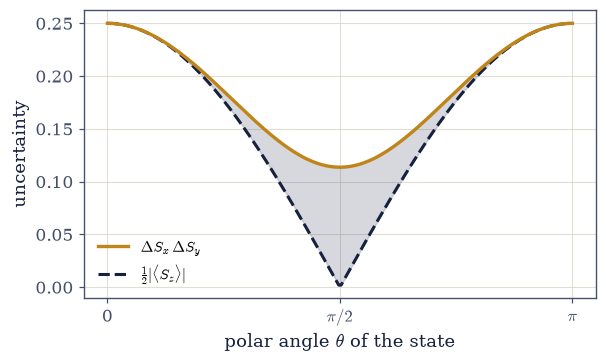
Fig. 520 The uncertainty relation is a state-dependent trade-off. Across a family of qubit states (sweeping the polar angle \(\theta\) at a fixed azimuth), the uncertainty product \(\Delta S_x\,\Delta S_y\) (amber) never falls below the Robertson bound \(\tfrac12|\langle S_z\rangle|\) (ink); the shaded gap is the slack. The bound itself moves with the state — it is largest where the atom is most definite along \(z\) (the poles, \(\theta=0,\pi\)), and there the product saturates, touching the bound exactly. Uncertainty is not a fixed number stamped on the observables; it is a trade-off whose floor each state sets through \(\langle S_z\rangle\). The principle is the inequality, true everywhere; the minimum-uncertainty states are where it becomes an equality.

Exercise 5 — Minimum-uncertainty states

The relation is an inequality, but for special states it closes into an equality. The \(\sigma_z\)-eigenstate \(|{+}z\rangle\) is one of them: it saturates the spin uncertainty relation, \(\Delta S_x\,\Delta S_y=\tfrac12|\langle S_z\rangle|=\tfrac14\) Eq. 525, which is the smallest product the pair \((S_x,S_y)\) permits any state at all. Such minimum-uncertainty states are the most “classical” ones quantum mechanics allows; the Gaussian wave packet is their position–momentum analogue (§6.9).

1. For \(|{+}z\rangle\), compute \(\Delta S_x\) and \(\Delta S_y\) with the dispersion helper and their product.

2. Compute the bound \(\tfrac12|\langle S_z\rangle|\) with the robertson_rhs you wrote in Exercise 3.

3. Confirm product and bound are equal (\(\tfrac14=\tfrac14\)) — a minimum-uncertainty state.

4. Note that a generic state (e.g. \(\theta=1,\varphi=1\), from the qubit you built in Exercise 4) does not saturate, leaving slack.

|+z⟩:  ΔSx·ΔSy = 0.2500,  ½|⟨Sz⟩| = 0.2500   saturated: True
generic (θ=1,φ=1):  ΔSx·ΔSy = 0.1572,  ½|⟨Sz⟩| = 0.1351   slack: 0.0222

Validation 5

✓  |+z⟩ saturates the uncertainty relation, ΔSx·ΔSy = ½|⟨Sz⟩| = ¼ — a minimum-uncertainty state   [got 0.25 vs expected 0.25 (rtol=1e-12, atol=1e-09)]

True

Exercise 6 — Compatible observables and a complete set

When observables commute the trade-off disappears altogether: they can be simultaneously sharp, and their joint eigenvalues label states Eq. 523, Eq. 526. \(S_z\) and \(S_z^2\) are the simplest such pair — any function of an observable commutes with it — and a maximal set of mutually commuting observables, a complete set of commuting observables, labels every state of a system uniquely.

1. Compute \([S_z,S_z^2]\) with the commutator helper (S_Z @ S_Z for \(S_z^2\)) and confirm it is the zero matrix (numpy.allclose).

2. Confirm both \(\Delta S_z\) and \(\Delta S_z^2\) are zero in \(|{+}z\rangle\) with the dispersion helper — both perfectly definite.

3. Note that the commuting bound \(\tfrac12|\langle[S_z,S_z^2]\rangle|=0\) — your Exercise 3 robertson_rhs returns zero here — so the relation is trivially satisfied, with no trade-off.

4. Reason in prose: joint eigenstates of commuting observables carry joint eigenvalue labels, and a complete set of commuting observables labels every state uniquely — the way the hydrogen atom’s states are tagged by \((n,\ell,m,m_s)\) in §6.17. That labelling is how quantum states are catalogued.

[Sz, Sz²] = 0 (compatible): True
in |+z⟩:  ΔSz = 0.00e+00,  ΔSz² = 0.00e+00   (both definite)
½|⟨[Sz,Sz²]⟩| = 0.00e+00   (zero: no uncertainty trade-off)
→ commuting observables carry joint eigenvalue labels; a complete set labels states uniquely (e.g. hydrogen's n,ℓ,m,m_s, §6.17).

Validation 6

✓  compatible observables ([Sz,Sz²]=0) can be simultaneously definite (both sharp in |+z⟩) and jointly label states

True

Exercise 7 — The general uncertainty relation in a larger space (student)

The relation is universal — it holds for any pair of observables on any space, not just spins, because its proof used nothing beyond the inner product Eq. 524. Random Hermitian observables on \(\mathbb{C}^3\) are therefore a fair and unsentimental test of it, and the saturation ratio \(\tfrac12|\langle[A,B]\rangle|/(\Delta A\,\Delta B)\), which lies in \([0,1]\), says how near such a state comes to the floor.

1. Build Hermitian \(A,B\) on \(\mathbb{C}^3\) (symmetrize random complex matrices, M + M.conj().T) and a normalized random state.

2. Compute \(\Delta A\), \(\Delta B\) with the dispersion helper and the bound with the robertson_rhs you wrote in Exercise 3.

3. Confirm \(\Delta A\,\Delta B\ge\tfrac12| \langle[A,B]\rangle|\) and report the saturation ratio.

4. Observe that the ratio is usually well below \(1\) — the bound is loose unless the state is special. The inequality is universal, but only rarely tight.

ΔA·ΔB = 3.0048 ≥ ½|⟨[A,B]⟩| = 0.8538:  holds = True
saturation ratio = 0.284   (≪ 1: the bound is loose for a generic state)

Validation 7

✓  the Robertson uncertainty relation holds for an arbitrary pair of Hermitian observables on ℂ³, with a saturation ratio in [0,1]

True

Exercise 8 — The uncertainty principle is an algebraic fact (synthesis)

The strangeness of the sequential Stern–Gerlach experiment was never about disturbing delicate atoms. It was the algebra. Two observables that fail to commute cannot both be sharp in any state, and how sharply they can be co-defined is bounded below by their commutator: \(\Delta A\,\Delta B\ge \tfrac12|\langle[A,B]\rangle|\). The Pauli matrices made this concrete — the three spin components pairwise anticommute and fail to commute, so definiteness along one axis forces maximal uncertainty along the others — and Cauchy–Schwarz, the same inequality that bounded amplitudes in §6.1, made it general. Minimum-uncertainty states saturate the bound; commuting observables escape it entirely and can be jointly sharp, labelling states by their joint eigenvalues.

There is no new computation to do here; the theorem is the result. “You cannot know both at once” sounds like a limitation imposed on us by clumsy instruments. It is the opposite — a fact about the observables themselves, true whether or not anyone is looking, and we derived it in three lines from the geometry of the Hilbert space. The next notebook (§6.7) finally sets the state in motion: the dynamics postulate worked out, the Hamiltonian generating unitary evolution, and the spin precessing on the very Bloch sphere this uncertainty trade-off lives on.

Notebook summary

The algebra behind the incompatibility that Stern–Gerlach showed and the variance measured — and the uncertainty principle as its theorem.

• The Pauli algebra Eq. 521, Eq. 522: \([\sigma_x,\sigma_y]=2i\sigma_z\) (cyclic), \(\{\sigma_i,\sigma_j\}=0\), \(\sigma_i^2=I\), \(\sigma_i\sigma_j=\delta_{ij}I+i\varepsilon_{ijk} \sigma_k\) — equivalently \([S_x,S_y]=iS_z\), the angular-momentum algebra.

• Compatibility Eq. 523: \([A,B]=0\) means jointly sharp; \([A,B]\ne0\) means not — and \(\sigma_x\) is maximally uncertain (\((\Delta\sigma_x)^2=1\)) in a \(\sigma_z\)-eigenstate.

• The Robertson relation, derived Eq. 524: \(\Delta A\,\Delta B\ge\tfrac12|\langle[A,B] \rangle|\), from Cauchy–Schwarz (§6.1) plus the commutator/anticommutator split — a theorem about operators, true of every state, not measurement disturbance.

• Minimum-uncertainty states Eq. 525: \(|{+}z\rangle\) saturates \(\Delta S_x\,\Delta S_y =\tfrac14=\tfrac12|\langle S_z\rangle|\) — the most classical states allowed.

• Complete sets Eq. 526: commuting observables can be jointly sharp and label states by joint eigenvalues (hydrogen’s \(n,\ell,m,m_s\), §6.17).

The uncertainty principle is Cauchy–Schwarz plus non-commutation. The commutator is literally the floor on how much two observables must trade off — an algebraic fact, true whether or not anyone looks.

Outlook

• Time evolution (§6.7): the Hamiltonian as generator, \(U(t)=e^{-iHt/\hbar}\), spin precession and Rabi oscillations — the state set in motion.

• The Bloch sphere (§6.8): the geometry of qubit states, where this uncertainty trade-off is visible.

• Position and momentum (§6.9): \([x,p]=i\hbar\) gives \(\Delta x\,\Delta p\ge\hbar/2\), with the Gaussian as the minimum-uncertainty state.

• The angular-momentum algebra generalized (§6.14): \([J_i,J_j]=i\hbar\varepsilon_{ijk}J_k\), the full theory of spin and orbital angular momentum, and complete sets of commuting observables (§6.17).

• Cross-reference §6.1 (Cauchy–Schwarz), §6.2 (commutators / common eigenbasis), §6.4 (the experiment), §6.5 (variance), and forward to §6.7, §6.8, §6.9, §6.14, §6.17.

Take this notebook with you

Use the download button (↓) in the toolbar above to save this notebook and run it yourself. The published notebooks ship without worked solutions; if you would like the reference solutions — to teach from or to check your own work — get in touch: hello@ramador.me.