6.10 The Schrödinger Equation as a PDE, Solved on a Computer

6.10 The Schrödinger Equation as a PDE, Solved on a Computer#

    Elementary Computational Physics
  

Volume VI — Quantum Mechanics Notebook 6.10

Diagonalize, and you are done. The time-independent Schrödinger equation is an eigenvalue problem for a Hermitian operator, and on a grid that operator is a matrix — the kinetic energy a finite-difference stencil, the potential a diagonal. We hand it to the same routine that diagonalized every operator in Movement 0, check it against the square well's exact spectrum, and then solve potentials no formula can reach.

Level · advanced • Est. · 160–195 min

    Raymond Amador
    v1.4.0  ·  2026-07-31  · 
          CC BY 4.0 (text) / MIT (code)
  

Notebook overview#

Volume VI has made one claim more than any other: quantum mechanics is linear algebra. In this notebook that claim stops being a slogan and becomes a literal method for solving real, continuous systems. The time-independent Schrödinger equation \(\hat H\psi=E\psi\) is, word for word, the eigenvalue problem of a Hermitian operator — the same problem we solved for a \(2\times2\) spin operator in §6.2. The only new step is to write that operator as a matrix, and the position representation of §6.9 tells us exactly how: put \(x\) on a grid, approximate the second derivative by a finite-difference stencil, and the Schrödinger operator becomes a finite matrix we hand to numpy.linalg.eigh. Its eigenvalues are the allowed energies; its eigenvectors are the stationary states.

The discipline of computational physics is to never trust a number you have not checked, so we begin with the one problem that has a clean exact answer — the infinite square well, \(E_n=n^2\pi^2\hbar^2 /2mL^2\) — and validate the method against it from three angles: the energies match to several digits, the eigenfunctions match the analytic sines \(\sqrt{2/L}\sin(n\pi x/L)\) to machine precision, and the computed states are orthonormal (the eigh guarantee of §6.2, now producing wave functions). We then watch the energy error fall as \(1/N^2\) with the grid resolution — the second-order accuracy of the finite-difference stencil, the floating-point-and-discretization sensibility of Volume 0 in the quantum setting — and are honest about where the method strains (the highest computed levels are always the least trustworthy).

Then comes the payoff. Nothing in the recipe used the square well’s analytic solution: it needs only \(V(x)\) on a grid. So the same three lines — build the kinetic stencil, add the diagonal potential, diagonalize — solve any one-dimensional potential, including those with no closed form. We turn them loose on an anharmonic well and read its spectrum straight off the screen. This is the engine for the rest of Movement II: bound states (§6.11), the harmonic oscillator (§6.12), and — once we restore the time dependence — wave packets in motion (§6.13).

As in every Volume VI notebook, each exercise opens with a crystal-clear statement and enumerated parts, each naming the exact operation — the \((1,-2,1)/dx^2\) second-difference stencil, numpy.diag to assemble the tridiagonal kinetic matrix, and numpy.linalg.eigh (the symmetric/Hermitian solver, returning sorted real eigenvalues and orthonormal eigenvectors).

Conventions. We set \(\hbar=1\) and \(m=1\). The grid is the interior of \([0,L]\) (or \([-L/2,L/2]\) for confining potentials): \(N\) points with spacing \(dx\), and the Dirichlet boundary condition \(\psi=0\) at the walls is built in by leaving the boundary points off the grid (a confining \(V\) instead needs a box large enough that \(\psi\) has decayed). Eigenfunctions from numpy.linalg.eigh are normalized in the discrete sense; we divide by \(\sqrt{dx}\) so that \(\int|\psi|^2dx=1\). For large grids scipy.linalg.eigh_tridiagonal is the efficient specialized solver. See Griffiths and Sakurai & Napolitano (the square well); Giordano & Nakanishi (the matrix method); and Notebooks §6.2 (eigh, the eigenvalue problem), §6.7 (stationary states), §6.9 (the position representation), and Volume 0 (finite differences, discretization error).

Theory in brief#

The time-independent Schrödinger equation as an eigenproblem#

Separating the time dependence (the stationary states \(e^{-iEt/\hbar}\) of §6.7) leaves the time-independent Schrödinger equation, an eigenvalue problem for a Hermitian operator,

(544)#\[\hat H\psi=E\psi,\qquad \hat H=-\frac{\hbar^2}{2m}\frac{d^2}{dx^2}+V(x) .\]

Its eigenvalues are the allowed energies and its eigenfunctions the stationary states. “Solving quantum mechanics” for a potential means diagonalizing this operator (§6.2).

Discretizing the Hamiltonian into a matrix#

Put \(x\) on a grid of \(N\) points with spacing \(dx\). The second derivative becomes the finite-difference stencil, a tridiagonal matrix,

(545)#\[\psi''(x_i)\approx\frac{\psi_{i+1}-2\psi_i+\psi_{i-1}}{dx^2},\qquad \hat H\to H=-\frac{\hbar^2}{2m}\,\frac{1}{dx^2}\,\mathrm{tridiag}(1,-2,1)+\mathrm{diag}\,V(x_i) .\]

So \(\hat H\) becomes a real symmetric matrix (Hermitian), and numpy.linalg.eigh returns its sorted eigenvalues (the energies) and orthonormal eigenvectors (the stationary states, normalized by dividing by \(\sqrt{dx}\)). The Dirichlet condition \(\psi=0\) at hard walls is built in by restricting to the interior grid.

The infinite square well: the validation#

For \(V=0\) in \([0,L]\) with infinite walls, the exact spectrum and eigenfunctions are

(546)#\[E_n=\frac{n^2\pi^2\hbar^2}{2mL^2},\qquad \psi_n(x)=\sqrt{\frac{2}{L}}\sin\frac{n\pi x}{L},\qquad n=1,2,\dots\]

The ground-state energy is nonzero — the zero-point energy: confinement forces motion, the uncertainty principle of §6.9 in action. We validate the numerics against all of this.

Convergence and its limits#

The finite-difference second derivative is second-order accurate, so the energy error falls as

(547)#\[|E_n^{\text{num}}-E_n|\sim\frac{1}{N^2} .\]

Higher levels (more wiggly eigenfunctions) need more points per wavelength and converge later — the highest computed eigenvalues are always the least trustworthy, a resolution diagnostic to state honestly.

The general method#

Nothing in the recipe used the analytic solution — it needs only \(V(x)\) on a grid,

(548)#\[\text{any } V(x)\ \xrightarrow{\ \text{stencil}+\mathrm{diag}\,V+\texttt{eigh}\ }\ \{E_n,\psi_n\} ,\]

so the same three steps solve any one-dimensional potential, including those with no closed form. This is the payoff: the computer solves problems pencil-and-paper cannot.

Setup#

Data and instruments only: the series palette, the unit conventions \(\hbar=m=1\), and plot_levels, the plotting scaffold that draws the standard textbook spectrum picture — each eigenfunction ribboned at its own energy above the potential. The two objects this notebook is named for are deliberately absent: you assemble the discretized Hamiltonian yourself in Exercise 1 and write the diagonalization that turns it into energies and stationary states in Exercise 2, and every later exercise calls the ones you wrote.

The Setup below holds this notebook’s data and instruments — nothing you are asked to build. It is collapsed so the building stays yours; expand it whenever you want the details.

Exercise 1 — Building the Hamiltonian matrix#

Everything in this notebook rests on a single translation: once \(x\) lives on a grid, the Schrödinger operator \(\hat H=-\tfrac{\hbar^2}{2m}\tfrac{d^2}{dx^2}+V(x)\) is a matrix Eq. 544, Eq. 545. The second derivative becomes the \((1,-2,1)/dx^2\) second-difference stencil — a tridiagonal matrix — and the potential becomes the diagonal \(\mathrm{diag}\,V(x_i)\), so \(H=-\tfrac{\hbar^2}{2m}\tfrac{1}{dx^2}\,\mathrm{tridiag}(1,-2,1)+\mathrm{diag}\,V\). Both pieces are real and symmetric, which is exactly what makes \(H\) Hermitian and licenses handing it to the Hermitian eigensolver of §6.2.

Write hamiltonian(x, V), returning \(H\) for a grid x and a potential V sampled on it: the kinetic term is \(-\hbar^2/2m\) times the \((1,-2,1)/dx^2\) stencil assembled with numpy.diag (\(-2\) on the main diagonal, \(1\) on the two off-diagonals), and the potential enters as numpy.diag(V). Write this one yourself — the implementation is the lesson.
Set up the interior grid for the square well (\(N\) points on \([0,L]\) with the two boundary points left off, which imposes \(\psi=0\) at the walls) with \(V=0\) inside, and assemble \(H\) on it.
Confirm \(H\) is real (numpy.isreal) and symmetric (\(H=H^{\mathsf T}\), numpy.allclose(H, H.T)) — a Hermitian operator. The Schrödinger operator is a matrix.

H shape (400, 400), real True, symmetric H = Hᵀ True
diagonal entries = −ℏ²/2m · (−2/dx²) + V = 160801.00;  off-diagonal = −ℏ²/2m · (1/dx²) = -80400.50

Validation 1#

✓  the discretized Hamiltonian is a real symmetric (Hermitian) matrix: −(ℏ²/2m)·(1,−2,1)/dx² stencil plus diag(V)

True

Exercise 2 — The infinite square well spectrum#

Never trust a number you have not checked, so the method’s first outing is on the one problem with a classroom-exact answer: for \(V=0\) between infinite walls the spectrum is \(E_n=n^2\pi^2\hbar^2/2mL^2\) Eq. 546. Everything the rest of the notebook does rests on this validation against an exact answer. Two features are worth watching. The ground state has \(E_1>0\) — the zero-point energy: a confined particle cannot be at rest, the uncertainty principle of §6.9 in action. And the relative errors grow with \(n\), because a wigglier eigenfunction gets fewer grid points per wavelength; Exercise 4 makes that quantitative.

Write solve(x, V): assemble \(H\) with the hamiltonian you wrote in Exercise 1, diagonalize it with numpy.linalg.eigh — the Hermitian solver of §6.2, which returns sorted real eigenvalues and orthonormal eigenvectors — and divide the eigenvector columns by \(\sqrt{dx}\) so each stationary state has \(\int|\psi_n|^2dx=1\). Return the energies and the states.
Run it on the square well of Exercise 1 (\(V=0\) on the interior grid) and take the lowest five eigenvalues.
Compare to \(E_n=n^2\pi^2\hbar^2/2mL^2\) for \(n=1,\dots,5\) and report the relative errors.
Report the ground-state energy and confirm \(E_1>0\).

n   E_numeric    E_exact      rel. error
   4.93478     4.93480    5.11e-06
  19.73880    19.73921    2.05e-05
  44.41118    44.41322    4.60e-05
  78.95037    78.95684    8.18e-05
 123.35428   123.37006    1.28e-04

ground-state energy E_1 = 4.93478 > 0  (zero-point energy: confinement forces motion)

Validation 2#

✓  the infinite square well spectrum is Eₙ = n²π²ℏ²/2mL² (validated against the exact answer)   [max|Δ| = 0.0157746 (rtol=0.001, atol=1e-09)]

True

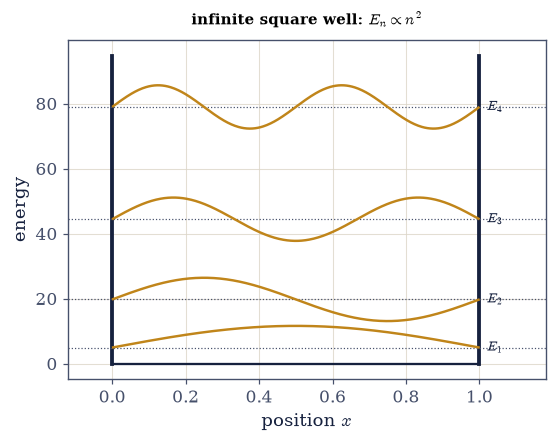
../../_images/bde2f3c8ab7a3847aef5a89321ede1decc45537694c250709c26024d442d5f14.png — Fig. 531 **The infinite square well, solved.** The flat potential (\(V=0\) between hard walls, ink) with the lowest four computed energy levels drawn as dotted lines and their stationary states \(\psi_n(x)\) (amber) riding at their energies. The levels climb as \(E_n\propto n^2\) — the spacing widens with \(n\) — and the lowest, \(E_1=\pi^2\hbar^2/2mL^2\), sits *above* the floor of the well: a confined particle has irreducible zero-point motion. Every number here came from handing a tridiagonal matrix to `numpy.linalg.eigh`, the same routine that diagonalized a spin operator in Movement 0; the wave functions are just its eigenvectors.#

Exercise 3 — The eigenfunctions#

The columns eigh returned are not merely numbers that pass a test: they are the stationary states themselves, and for the square well their closed form is known, \(\psi_n(x)=\sqrt{2/L}\sin(n\pi x/L)\) Eq. 546. An eigenvector is defined only up to a global sign, and a solver may return either, so a comparison against the analytic form has to fix that convention before it means anything. Beyond matching the sines, the states inherit the eigh orthonormality of §6.2, \(\langle\psi_i|\psi_j\rangle= \delta_{ij}\) — the same guarantee that held for spin vectors there, now producing wave functions.

Extract \(\psi_n(x)\) from the output of the solve you wrote in Exercise 2 (already normalized by \(\sqrt{dx}\)).
Fix the sign convention: flip so the overlap with the analytic form is positive.
Compare to \(\sqrt{2/L}\sin(n\pi x/L)\) with numpy.max(numpy.abs(...)).
Verify orthonormality — the discrete inner product (states.T @ states)·dx is the identity to machine precision.

max|ψ_numeric − ψ_analytic| for n=1,2,3:  6.57e-13  (machine precision)
orthonormality max|⟨ψ_i|ψ_j⟩ − δ_ij|:  1.78e-15  (the eigh guarantee, now wave functions)

Validation 3#

✓  the eigenfunctions are √(2/L)sin(nπx/L) and orthonormal (⟨ψ_i|ψ_j⟩=δ_ij to machine precision)   [max|Δ| = 6.5728e-13 (rtol=1e-06, atol=1e-09)]

True

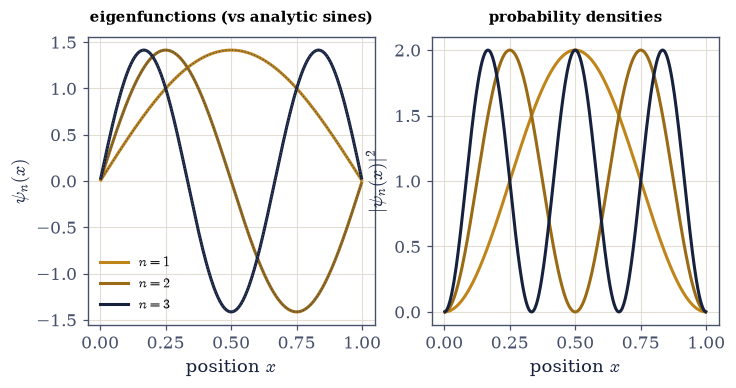
../../_images/58f74ed160d66dac6cd4a2c6695b261b685c685fd54d49c28bba041cfe652dda.png — Fig. 532 **The stationary states and their densities.** Left: the first three eigenfunctions \(\psi_n(x)\) of the square well — the computed states (amber) lie exactly on the analytic sines \(\sqrt{2/L}\sin(n\pi x/L)\) (dotted), with \(n-1\) interior nodes apiece. Right: the probability densities \(|\psi_n(x)|^2\), the likelihood of finding the particle at each point. These are nothing but the eigenvectors `numpy.linalg.eigh` returned — orthonormal to machine precision, exactly as they were for the spin operators of Movement 0 — read now as functions of position. Diagonalization did not change; only the size of the matrix did.#

Exercise 4 — Convergence with grid resolution#

The finite-difference second derivative is second-order accurate, so the energy error should fall as \(1/N^2\) with the number of grid points Eq. 547: a slope of \(-2\) on log–log axes, a fourfold gain for every doubling of the resolution. That is what makes the error respectable rather than mysterious — it is discretization error, controllable and predictable, exactly the sensibility of Volume 0 in quantum dress. Higher levels ride above the line and converge later, since the wigglier the eigenfunction the more grid points per wavelength it needs; the highest computed eigenvalue is always the least trustworthy.

Solve the square well for \(N=25,50,100,\dots,800\) with the solve you wrote in Exercise 2.
Compute the relative error of the ground-state energy \(E_1\) against the exact \(\pi^2\hbar^2/2mL^2\).
Plot the error versus \(N\) on log–log axes and confirm the slope is \(-2\) (a \(1/N^2\) reference line).

N      relative error of E_1
 1.22e-03
 3.16e-04
 8.06e-05
 2.04e-05
 5.11e-06
 1.28e-06

log–log slope = -1.980  (≈ −2: second-order convergence, error ~ 1/N²)

Validation 4#

✓  the finite-difference method converges at second order: the ground-state energy error scales as ~1/N²   [got -1.97953 vs expected -2 (rtol=1e-06, atol=0.1)]

True

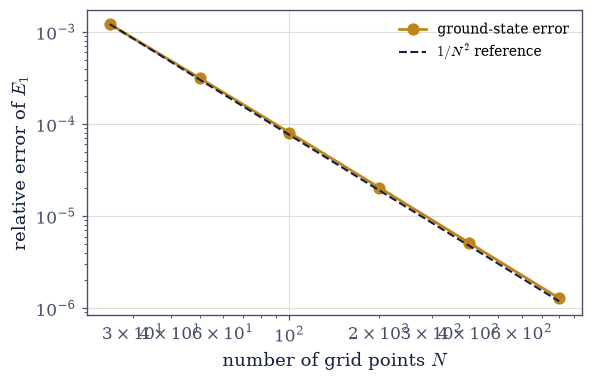
../../_images/4260af75fc88672c377a7238fa6f271e13b53e311e6c6803c5f069aa66725fa1.png — Fig. 533 **Second-order convergence.** The relative error in the computed ground-state energy of the square well against the number of grid points \(N\), on log–log axes (amber dots), with a \(1/N^2\) reference slope (dashed). The points fall on a line of slope \(-2\): doubling the resolution cuts the error fourfold, the hallmark of the second-order \((1,-2,1)\) finite-difference stencil. The error is not mysterious — it is discretization error, predictable and controllable, exactly the floating-point sensibility of Volume 0 in the quantum setting. Higher levels, whose wave functions wiggle more, ride above this line and converge later; the highest computed eigenvalue is always the least trustworthy.#

Exercise 5 — A potential with no closed form#

Nothing in the recipe used the square well’s analytic solution — it needs only \(V(x)\) sampled on a grid Eq. 548, so the same three steps solve potentials with no closed form at all, which is to say the overwhelming majority of them. The anharmonic well \(V(x)=\tfrac12x^2+\lambda x^4\) is one such potential, and it wears its anharmonicity where the spectrum can be read: the quartic term steepens the walls, squeezing the higher states upward, so the level spacings \(E_{n+1}-E_n\) increase with \(n\) instead of staying equal as a harmonic oscillator’s would. The one precaution a confining potential demands is a box wide enough that the states of interest have decayed before the hard walls.

Choose \(V(x)=\tfrac12x^2+\lambda x^4\) on a box \([-L/2,L/2]\) large enough that the low-lying wave functions decay to zero at the edges.
Build \(H\) and diagonalize with the same solve you wrote in Exercise 2 — nothing about the recipe changes.
Report the lowest five energies.
Confirm the level spacings \(E_{n+1}-E_n\) increase with \(n\), an anharmonicity no two-term formula captures. The method needs only \(V(x)\); the computer solves the unsolvable.

anharmonic well V = ½x² + 0.3x⁴, lowest five energies:
  [0.638  2.0945 3.8443 5.7954 7.9095]
  level spacings E_{n+1}−E_n = [1.4565 1.7498 1.9511 2.1142]
  (a harmonic oscillator would give equal spacings of 1; here they grow — anharmonicity)

Validation 5#

✓  the finite-difference eigenmethod solves an arbitrary potential: the anharmonic well has growing level spacings and orthonormal eigenfunctions

True

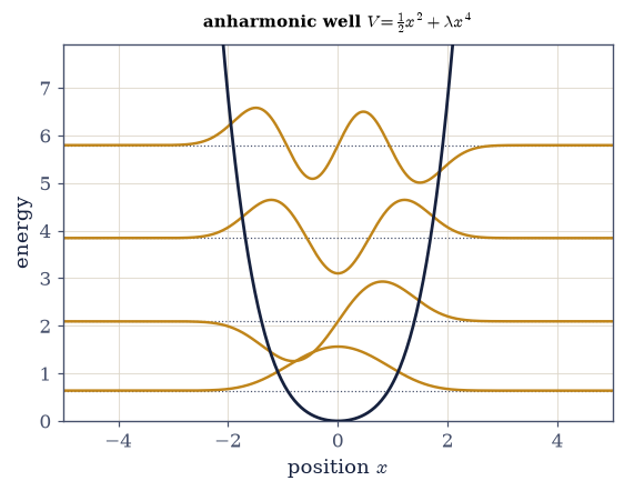
../../_images/2808b41fa089694fafda5d25d7e55cf8ccb9c33d90c97871e7e120076c7e6e9b.png — Fig. 534 **A potential no formula can reach.** The anharmonic well \(V(x)=\tfrac12x^2+\lambda x^4\) (ink) with its lowest four computed energy levels (dotted) and stationary states (amber) — obtained from the *same* three lines that solved the square well, because the method needs only \(V(x)\) on a grid. The quartic term steepens the walls, so the levels are not equally spaced as a harmonic oscillator’s would be: each gap is *wider* than the last. This is the engine of computational quantum mechanics — hand it any potential and it returns the spectrum and the states, including for the overwhelming majority of potentials that have no closed-form solution at all.#

Exercise 6 — Resolution, box size, and trusting the answer (student)#

A computed eigenvalue is only as good as its grid and its box Eq. 547, Eq. 548, and for a confining potential the two err in different directions. Too small a box adds artificial confinement — the hard walls squeeze the state and push its energy up — while too coarse a grid fails to resolve the wave function’s wiggles. The harmonic oscillator \(V=\tfrac12x^2\) is the honest test bed for both, since its exact spectrum \(E_n=n+\tfrac12\) is known and each error can be watched shrinking against it.

Solve \(V=\tfrac12x^2\) at several box sizes \(L\) (with the grid fine enough) with the solve you wrote in Exercise 2, and read the ground-state energy.
Show that too small a box raises the energy and that it converges to \(\tfrac12\) as \(L\) grows.
Separately, show that too coarse a grid (small \(N\)) also errs, converging as \(N\) grows.
State the rule of thumb: the box must contain the wave function’s decay, and the grid must resolve its wiggles (points per wavelength). The computational-physics discipline is to trust an eigenvalue only inside its converged window.

box size L (fixed dx≈0.02):  E_1 → ½
  L =    3:  E_1 = 0.67794   (error 1.8e-01)
  L =    5:  E_1 = 0.50451   (error 4.5e-03)
  L =    8:  E_1 = 0.49999   (error 1.2e-05)

  L =   14:  E_1 = 0.49999   (error 1.3e-05)
grid points N (fixed box L=14):  E_1 → ½
  N =   50:  E_1 = 0.49744   (error 2.6e-03)
  N =  100:  E_1 = 0.49937   (error 6.3e-04)
  N =  300:  E_1 = 0.49993   (error 6.9e-05)
  N =  700:  E_1 = 0.49999   (error 1.3e-05)

converged (L=16, N=800): E_1..E_4 = [0.5    1.4999 2.4998 3.4997]  vs exact n+½ = [0.5, 1.5, 2.5, 3.5]

Validation 6#

✓  a trustworthy eigenvalue requires an adequate box and grid: with both converged, the harmonic oscillator gives Eₙ = n + ½   [max|Δ| = 0.000313311 (rtol=1e-06, atol=0.01)]

True

Exercise 7 — Wave mechanics is a matrix eigenvalue problem (synthesis)#

The time-independent Schrödinger equation is the eigenvalue problem of a Hermitian operator, and on a grid that operator is a matrix we already knew how to diagonalize. We checked the recipe against the square well’s exact spectrum — energies to several digits, eigenfunctions to machine precision, orthonormality from eigh — watched the error fall as \(1/N^2\), and then solved a potential no formula can reach, all with the same three lines that diagonalized a \(2\times2\) spin operator in Movement 0: build the kinetic stencil, add the diagonal potential, call numpy.linalg.eigh. This is the engine of computational quantum mechanics: give it a potential, get its spectrum and its stationary states.

There is no new computation to do here; the method is the result. And there is a quiet triumph in it. The equation that took Schrödinger a winter to solve for hydrogen, we solve for an arbitrary potential in a few lines — not because we are cleverer, but because diagonalizing a matrix is something a computer does without thinking. The next notebooks apply this engine to real bound-state problems and parity (§6.11) and to the harmonic oscillator’s analytic and algebraic solutions checked against the grid (§6.12); and once we restore the time dependence, to wave packets in motion (§6.13). The arena is the continuum now, but the method has not changed since §6.2 — diagonalize.

Notebook summary#

The Schrödinger equation solved by the diagonalization method of Movement 0 — the engine of computational quantum mechanics.

The eigenproblem Eq. 544: \(\hat H\psi=E\psi\) with \(\hat H=-\tfrac{\hbar^2}{2m}\tfrac{d^2} {dx^2}+V\) — the Hermitian eigenvalue problem of §6.2, now for a continuous system.
Discretization Eq. 545: the \((1,-2,1)/dx^2\) stencil (numpy.diag) makes the kinetic term tridiagonal and \(V\) diagonal, so \(\hat H\to\) a real symmetric matrix for numpy.linalg.eigh (scipy.linalg.eigh_tridiagonal for speed).
The square-well validation Eq. 546: energies \(E_n=n^2\pi^2\hbar^2/2mL^2\) to several digits, eigenfunctions \(\sqrt{2/L}\sin(n\pi x/L)\) to machine precision, orthonormal; a nonzero zero-point energy.
Convergence Eq. 547: second-order, error \(\sim1/N^2\) (slope \(-2\) on log–log); higher levels converge later — the highest are least trustworthy.
The general method Eq. 548: the recipe needs only \(V(x)\), so it solves any 1-D potential — demonstrated on an anharmonic well with growing level spacings.

Solving the Schrödinger equation is diagonalization. The arena changed from two amplitudes to a continuum; the method did not change at all.

Outlook#

Bound states in one dimension (§6.11): finite wells, parity, bound-state counting, the double well.
The harmonic oscillator (§6.12): the analytic and algebraic (ladder-operator) solutions, checked against the grid; coherent states.
Time evolution on the grid (§6.13): split-step Fourier and Crank–Nicolson for wave-packet dynamics.
Three dimensions and central potentials (§6.16–§6.17): separate variables and solve the radial equation the same way.
Cross-reference §6.2 (eigh, the eigenvalue problem), §6.7 (stationary states), §6.9 (the position representation), Volume 0 (finite differences, discretization error), and forward to §6.11, §6.12, §6.13.

Take this notebook with you

Use the download button (↓) in the toolbar above to save this notebook and run it yourself. The published notebooks ship without worked solutions; if you would like the reference solutions — to teach from or to check your own work — get in touch: hello@ramador.me.