6.5 The Postulates of Quantum Mechanics

6.5 The Postulates of Quantum Mechanics#

    Elementary Computational Physics
  

Volume VI — Quantum Mechanics Notebook 6.5

The rules, stated once. Everything the Stern–Gerlach experiment forced on us — states as vectors, observables as Hermitian operators, outcomes as eigenvalues with Born probabilities, measurement as collapse — becomes a short list of postulates. We state each one precisely, show it is the distilled content of something we already understood, and derive from it the two numbers a laboratory records: the expectation value and the uncertainty.

Level · intermediate • Est. · 150–180 min

    Raymond Amador
    v1.4.0  ·  2026-07-31  · 
          CC BY 4.0 (text) / MIT (code)
  

Notebook overview#

The last notebook let an experiment back us into quantum mechanics. This one writes down what we were backed into. Every rule we used to explain the Stern–Gerlach data — a state is a vector, an observable is a Hermitian operator, an outcome is an eigenvalue drawn with a certain probability, a measurement projects — is here stated once and for all as a postulate. There is no new physics in this notebook; the student has already seen each rule in action. What is new is the systematization: naming the rules, making them precise, and showing they fit together into a consistent whole. The entire edifice of quantum mechanics rests on the five short statements below.

The notebook is built on a single pedagogical spine: each postulate is introduced by recalling the Stern–Gerlach fact it explains, then stated formally, then verified computationally. No postulate is met cold. And every one is stated in the language Movement 0 built — states are the unit vectors of §6.1, observables the Hermitian operators of §6.2, measurement the projection of §6.3. This is where that arsenal proves its worth: the postulates are not new mathematics, only physics asserted about the mathematics we already have.

From the five postulates two derived quantities follow, and they are the bridge from the formalism to the laboratory: the expectation value \(\langle A\rangle=\langle\psi|A|\psi\rangle\), the mean of many measurements, and the variance \((\Delta A)^2=\langle A^2\rangle-\langle A\rangle^2\), their spread — the same mean and variance of a distribution from §5.2, now read off a quantum state. The variance vanishes exactly on eigenstates (the definite values), and it is the quantity the uncertainty relation of §6.6 will bound. We work throughout in the two-state system and small finite examples, where every postulate is a few lines of numpy.

As in every Volume VI notebook, each exercise opens with a crystal-clear statement and enumerated parts, each naming the exact operation — numpy.vdot for \(\langle\psi|A|\psi\rangle\), numpy.linalg.eigh for the spectral data, explicit projectors via numpy.outer, and numpy.random.default_rng for sampling outcomes.

The five postulates, in brief. (1) State: a physical state is a unit vector \(|\psi\rangle\) (a ray — global phase unphysical). (2) Observable: a measurable quantity is a Hermitian operator \(A\); its eigenvalues are the possible outcomes. (3) Born rule: outcome \(a_i\) occurs with probability \(|\langle a_i|\psi\rangle|^2=\langle\psi|P_i|\psi\rangle\). (4) Collapse: the state jumps to the normalized projection \(P_i|\psi\rangle/\|P_i|\psi\rangle\|\) onto the measured eigenspace (the Lüders rule). (5) Dynamics: between measurements \(i\hbar\,\partial_t|\psi\rangle =H|\psi\rangle\) — stated here, worked out in §6.7.

How to read the checks. Each exercise closes with a validate call: an observable’s eigenvalues as outcomes; the Born rule in its three equivalent forms, summing to one; the expectation value two ways; the variance non-negative and zero on eigenstates; collapse giving a repeatable definite value; and the degenerate (Lüders) case projecting onto a whole eigenspace. A ✓ is strong evidence; a ✗ is a prompt to locate the discrepancy.

Conventions and scope. Unit states; Hermitian observables; \(\hbar=1\) unless shown. The dynamics postulate is stated but its working-out (the time-evolution operator, precession, Rabi) is §6.7; the uncertainty relation that bounds \(\Delta A\) is §6.6; the Bloch-sphere geometry is §6.8; mixed states and the density matrix are §6.26. See Sakurai & Napolitano (§1.3–1.4); Nielsen & Chuang; and Notebooks §6.1 (states), §6.2 (observables), §6.3 (projectors), §6.4 (the experiment), §5.2 (expectation and variance).

Theory in brief#

Postulate 1 — the state#

Recall (§6.4): the Stern–Gerlach atom was a vector in \(\mathbb{C}^2\). Formally,

(514)#\[\text{a physical state is a unit vector }|\psi\rangle,\quad \langle\psi|\psi\rangle=1,\quad |\psi\rangle\simeq e^{i\gamma}|\psi\rangle\ (\text{a ray}) .\]

States differing by a global phase are the same physical state (§6.1).

Postulate 2 — observables#

Recall (§6.4): \(S_z\), with outcomes \(\pm\hbar/2\) and definite-value states \(|{\pm}z\rangle\). Formally,

(515)#\[\text{a measurable quantity is a Hermitian operator }A=A^{\dagger};\ \text{its eigenvalues }a_i\ \text{are the possible outcomes},\]

and its orthonormal eigenvectors are the definite-value states (§6.2).

Postulate 3 — the Born rule#

Recall (§6.4): the \(\cos^2(\theta/2)\) law. Measuring \(A\) on \(|\psi\rangle\) gives \(a_i\) with

(516)#\[P(a_i)=|\langle a_i|\psi\rangle|^2=\langle\psi|P_i|\psi\rangle=\|P_i|\psi\rangle\|^2 ,\]

where \(P_i\) projects onto the \(a_i\)-eigenspace (§6.3). The probabilities sum to one because the projectors resolve the identity, \(\sum_iP_i=I\) (§6.3).

Postulate 4 — collapse#

Recall (§6.4): the projected \(|{+}x\rangle\) atom; the sequential experiment. Immediately after outcome \(a_i\),

(517)#\[|\psi\rangle\ \longrightarrow\ \frac{P_i|\psi\rangle}{\|P_i|\psi\rangle\|} .\]

A repeated measurement then gives \(a_i\) with certainty — repeatability, the condition that lets “the system has value \(a_i\) now” mean something. For a degenerate outcome the projection is onto the whole eigenspace (the Lüders rule), not a single eigenvector.

Postulate 5 — dynamics#

Between measurements the state evolves by the Schrödinger equation,

(518)#\[i\hbar\,\frac{\partial}{\partial t}|\psi\rangle=H|\psi\rangle,\]

with \(H\) the Hamiltonian (a Hermitian observable, the energy). We state it here as the fifth postulate; its solution — the unitary \(U(t)=e^{-iHt/\hbar}\) (the exponential map of §6.2, the function-of-operator of §6.3) — and its consequences (precession, Rabi) are developed in §6.7.

Derived — expectation and variance#

The mean of many measurements of \(A\) on identically-prepared states, and their spread, are

(519)#\[\langle A\rangle=\langle\psi|A|\psi\rangle=\sum_i a_i\,P(a_i)\quad(\text{real, since }A=A^{\dagger}),\]

(520)#\[(\Delta A)^2=\langle A^2\rangle-\langle A\rangle^2=\sum_i (a_i-\langle A\rangle)^2P(a_i)\ \ge 0,\]

the same mean and variance of a distribution as in §5.2. The variance vanishes exactly when \(|\psi\rangle\) is an eigenstate of \(A\) — a definite value — and \(\Delta A\) is what the uncertainty relation bounds (§6.6).

Setup#

The data are the series palette and the conventions this notebook computes in. The one piece of machinery here is already earned: the rank-1 projector \(|e\rangle\langle e|\), built from scratch in §6.3 and restated as a tool. Everything the postulates are is built where it is used — the eigenspace projectors, the Born probabilities and the expectation value in Exercise 3, the variance in Exercise 4, and the measurement-and-collapse sampler in Exercise 5.

The Setup below holds this notebook’s data and instruments — nothing you are asked to build. It is collapsed so the building stays yours; expand it whenever you want the details.

Exercise 1 — States and observables (Postulates 1 and 2)#

Recall from §6.4 that the spin-\(z\) atom is a unit vector in \(\mathbb{C}^2\) and \(S_z\) is the observable whose eigenvalues \(\pm\tfrac12\) are the possible outcomes. Postulates 1 and 2 state that in general: a legal state is any unit vector, a legal observable any Hermitian operator, its real eigenvalues are the possible outcomes and its orthonormal eigenvectors the definite-value states Eq. 514, Eq. 515. The specimen here is a random Hermitian \(A\) on \(\mathbb{C}^3\) with a random unit state — a larger arena than the qubit, so nothing about the two-state system is quietly doing the work.

Confirm \(|\psi\rangle\) is a unit vector, \(\langle\psi|\psi\rangle=1\), with numpy.vdot.
Confirm \(A\) is Hermitian, numpy.allclose(A, A.conj().T).
Diagonalize \(A\) with numpy.linalg.eigh: the (real) eigenvalues are the possible outcomes, the orthonormal eigenvectors the definite-value states.
Note the parallel to \(S_z\) in §6.4 — the same two-postulate structure, now in \(\mathbb{C}^3\).

⟨ψ|ψ⟩ = 1.000000  (unit state: True)
A Hermitian: True
possible outcomes (eigenvalues): [-2.4316  1.5851  3.0122]
definite-value states are the columns of the eigenvector matrix (orthonormal: True)

Validation 1#

✓  a state is a unit vector and an observable is a Hermitian operator whose real eigenvalues are the possible outcomes and whose orthonormal eigenvectors are the definite-value states

True

Exercise 2 — The Born rule and its three forms (Postulate 3)#

The Born rule is the quantitative content of the \(\cos^2(\theta/2)\) law of §6.4, and it wears three equivalent faces that the §6.3 dictionary makes interchangeable: the squared amplitude \(|\langle a_i|\psi\rangle|^2\), the projector expectation \(\langle\psi|P_i|\psi\rangle\), and the squared norm of the projected state \(\|P_i|\psi\rangle\|^2\) Eq. 516. That the three agree, and that the probabilities sum to one — a consequence of the resolution of the identity \(\sum_iP_i=I\) (§6.3) — is the postulate’s internal consistency, worth verifying rather than reciting. The state and observable are the ones from Exercise 1.

For each eigenvector \(|a_i\rangle\) compute \(P(a_i)=|\langle a_i|\psi\rangle|^2\) with numpy.abs(numpy.vdot(a_i, psi))**2.
Build the projector \(P_i=\)numpy.outer(a_i, numpy.conj(a_i)) and compute \(\langle\psi|P_i|\psi\rangle\) with numpy.vdot(psi, P_i @ psi).real.
Compute \(\|P_i|\psi\rangle\|^2\) with numpy.linalg.norm(P_i @ psi)**2.
Confirm all three agree for each outcome, and that \(\sum_i P(a_i)=1\).

|⟨a_i|ψ⟩|²       = [0.69704 0.29561 0.00736]
⟨ψ|P_i|ψ⟩       = [0.69704 0.29561 0.00736]
‖P_i|ψ⟩‖²       = [0.69704 0.29561 0.00736]
three forms agree: True;  Σ P(a_i) = 1.0000000000

Validation 2#

✓  the Born probability has three equivalent forms |⟨a_i|ψ⟩|² = ⟨ψ|P_i|ψ⟩ = ‖P_iψ‖², and they sum to one (ΣP_i = I)   [max|Δ| = 6.66134e-16 (rtol=1e-12, atol=1e-09)]

True

Exercise 3 — The expectation value (Postulate 3, derived)#

The expectation value is the bridge from the operator to the laboratory average — the mean reading of many measurements of \(A\) on identically-prepared states Eq. 519. It is real, because \(A\) is Hermitian, and it must agree with the ordinary mean \(\sum_i a_iP(a_i)\) of §5.2 — the same expectation of a distribution, now read off a quantum state.

Exercise 2 computed the Born probabilities by hand, one rank-1 projector at a time. From here on the notebook needs them packaged, and packaged in the form that survives degeneracy: when several eigenvectors share an eigenvalue, the probability of that outcome belongs to the projector onto the whole eigenspace, the sum of their rank-1 projectors (the form Exercise 6 puts to work). numpy.linalg.eigh returns the real eigenvalues and orthonormal eigenvectors of a Hermitian matrix (§6.2); eigenvalues equal to within a tolerance are the degenerate ones, and the Setup’s projector turns each eigenvector into its rank-1 projector (§6.3).

Write eigenspace_projectors(A, tol=1e-9), returning (eigenvalue, eigenspace projector) for each distinct eigenvalue of a Hermitian A: diagonalize with numpy.linalg.eigh, then add each eigenvector’s rank-1 projector into the group whose eigenvalue matches within tol, opening a new group when none does. Write this one yourself — the implementation is the lesson.
Write outcome_probabilities(A, psi), returning \((a_i, P(a_i))\) for each distinct eigenvalue with \(P(a_i)=\langle\psi|P_i|\psi\rangle\) (numpy.vdot(psi, P_i @ psi).real) — the eigenspace form of Eq. 516, correct even when the eigenvalue is degenerate.
Write expectation(A, psi), the expectation value \(\langle\psi|A|\psi\rangle\) (numpy.vdot(psi, A @ psi).real).
Compute \(\langle A\rangle\) with your expectation, for the state and observable of Exercise 1.
Compute \(\sum_i a_i P(a_i)\) from the eigenvalues and probabilities your outcome_probabilities returns.
Confirm the two agree, and that the imaginary part of \(\langle\psi|A|\psi\rangle\) is zero.

⟨A⟩ = ⟨ψ|A|ψ⟩      = -1.204194
⟨A⟩ = Σ a_i P(a_i) = -1.204194
agree: True;  ⟨A⟩ real (Im = 2.2e-16)

Validation 3#

✓  the expectation value ⟨A⟩ = ⟨ψ|A|ψ⟩ equals Σ a_i P(a_i), the laboratory average of many measurements (§5.2 in the quantum setting)   [got -1.20419 vs expected -1.20419 (rtol=1e-12, atol=1e-09)]

True

Exercise 4 — Variance and definite values (derived)#

The variance measures the spread of the outcomes — and it is the quantity the uncertainty relation (§6.6) will bound Eq. 520. Written as \(\langle A^2\rangle-\langle A\rangle^2\) it is a statement about operators; written as \(\sum_i(a_i-\langle A\rangle)^2P(a_i)\) it is the familiar spread of a distribution (§5.2), and the two must agree. It is never negative, and it vanishes exactly on an eigenstate of \(A\) — zero variance is what “a definite value” means, the \(|{\pm}z\rangle\) atoms of §6.4 being the case already met.

Write variance(A, psi), the variance \(\langle A^2\rangle-\langle A\rangle^2\), built from the expectation you wrote in Exercise 3 (expectation(A @ A, psi) - expectation(A, psi)**2).
Compute \((\Delta A)^2\) for the state and observable of Exercise 1, confirm it equals \(\sum_i(a_i-\langle A\rangle)^2P(a_i)\) from your Exercise 3 Born probabilities, and that it is \(\ge0\).
Evaluate the variance in an eigenstate of \(A\) (a column of numpy.linalg.eigh’s eigenvector matrix) and find it is zero — a state with a definite value.

(ΔA)² = ⟨A²⟩ − ⟨A⟩²        = 3.480826
(ΔA)² = Σ(a_i − ⟨A⟩)²P(a_i) = 3.480826   (≥ 0, forms agree: True)
variance in an eigenstate of A: 8.88e-16   (zero — a definite value)

Validation 4#

✓  the variance ⟨A²⟩−⟨A⟩² is non-negative, agrees with Σ(a_i−⟨A⟩)²P(a_i), and vanishes exactly on eigenstates (definite values)   [max|Δ| = 1.33227e-15 (rtol=1e-06, atol=1e-12)]

True

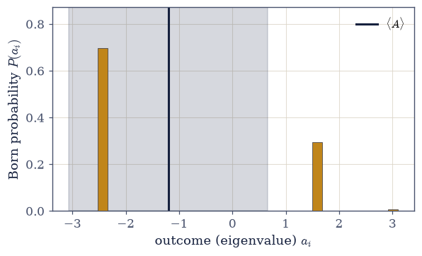
../../_images/644febac6b5b47e1481e446600d8403646d4348fced6969fc30387cfa0295097.png — Fig. 518 **The expectation and the uncertainty as the mean and spread of the outcome distribution.** Measuring the observable \(A\) on the state \(|\psi\rangle\) yields one of its eigenvalues \(a_i\) (horizontal axis), each with the Born probability \(P(a_i)\) (amber bars). The expectation value \(\langle A\rangle=\sum_i a_iP(a_i)\) (ink line) is the mean of this distribution, and the shaded band is \(\langle A\rangle\pm\Delta A\), one standard deviation set by the variance. This is exactly the mean-and-variance picture of §5.2, now read off a quantum state: the formalism’s \(\langle\psi|A|\psi\rangle\) and \(\langle A^2\rangle-\langle A\rangle^2\) are the two numbers a laboratory records.#

Exercise 5 — Collapse and repeatability (Postulate 4)#

Recall the sequential Stern–Gerlach experiment of §6.4: once an atom is measured, a repeat of the same measurement is certain. Postulate 4 states that in general Eq. 517 — an outcome \(a_i\) arrives with its Born probability and the state jumps to the normalized projection \(P_i|\psi\rangle/\|P_i|\psi\rangle\|\) onto the measured eigenspace. Collapse together with repeatability is what makes “the system has value \(a_i\) now” a meaningful statement, and repeatability is something to check rather than assume: in the collapsed state the expectation must be the value obtained, the variance must be zero, and the same outcome must recur with probability one.

Write measure(A, psi, rng), one simulated measurement: form the spectrum with your Exercise 3 eigenspace_projectors, collect the Born probabilities \(\langle\psi|P_i|\psi\rangle\), renormalize them against rounding, draw an index with rng.choice(len(spectrum), p=probs), and return the eigenvalue together with the collapsed state \(P_i|\psi\rangle/\|P_i|\psi\rangle\|\). Write this one yourself — the implementation is the lesson.
Sample an outcome \(a_i\) and its collapsed state with your measure, seeding numpy.random.default_rng(7).
Compute \(\langle A\rangle\) in the collapsed state with your Exercise 3 expectation — it equals the sampled \(a_i\) — and confirm your Exercise 4 variance is zero there.
Confirm re-measuring returns \(a_i\) with probability \(1\): its Born probability in the collapsed state, from your Exercise 3 outcome_probabilities.

sampled outcome a_i = -2.4316
⟨A⟩ in the collapsed state = -2.4316   (= a_i: True)
variance in the collapsed state = -8.88e-16   (definite value)
probability the repeat measurement gives a_i again = 1.0000   (certain)

Validation 5#

✓  measurement collapses the state onto the measured eigenspace, giving a definite value that a repeated measurement returns with certainty (repeatability)

True

Exercise 6 — Degenerate observables: the Lüders rule (Postulates 3 and 4)#

When an eigenvalue is degenerate — shared by more than one eigenvector — the Born rule and collapse use the projector onto the whole eigenspace, not a single eigenvector (the Lüders rule, the subtlety most first courses skip) Eq. 516, Eq. 517. This is the case your eigenspace_projectors of Exercise 3 was written to handle, and it is not a curiosity: degeneracy is the rule for the hydrogen atom, and the reason degenerate perturbation theory needs a chapter of its own later in the volume. A degenerate observable is easy to manufacture — conjugate a diagonal matrix carrying a repeated entry by a unitary, and the repeated eigenvalue’s eigenspace is the plane that unitary carries the corresponding coordinate plane onto.

Build \(B=2\,P_{\text{sub}}+5\,P_{\text{other}}\) with a 2-fold degenerate eigenvalue \(2\): form an orthonormal basis with numpy.linalg.qr and set \(B=Q\,\mathrm{diag}(2,2,5)\,Q^{\dagger}\) (Q @ numpy.diag([2,2,5]) @ Q.conj().T).
The probability of the value \(2\) is \(\langle\psi| P_{\text{eigenspace}}|\psi\rangle\), where \(P_{\text{eigenspace}}\) is the projector onto the whole 2-D eigenspace (the eigenspace_projectors you wrote in Exercise 3 sums the degenerate eigen-projectors).
The collapsed state is the normalized projection onto that eigenspace — not a single eigenvector.
Verify the collapsed state lies in the eigenspace by confirming \(\langle B\rangle=2\) there (your Exercise 3 expectation), and that the eigenspace projector has rank \(2\) (numpy.trace).

P(value 2) = ⟨ψ|P_eigenspace|ψ⟩ = 0.8083
⟨B⟩ in the collapsed state = 2.0000   (= 2, lies in the eigenspace)
rank of the eigenspace projector = 2   (the degenerate eigenspace is 2-D)

Validation 6#

✓  for a degenerate outcome the Born rule and collapse use the projector onto the whole eigenspace (the Lüders rule), not a single eigenvector

True

Exercise 7 — Reading a quantum state through measurements (student)#

The postulates say exactly what one measurement yields — and, by the same token, what it does not reveal. They fix one measurement; learning a state takes an ensemble. The specimen is the qubit \(|\psi\rangle=\cos\tfrac{\theta}{2}|{+}z\rangle+e^{i\varphi}\sin\tfrac{\theta}{2}|{-}z\rangle\) with \(\theta=1.0,\varphi=0.8\), measured with the observable \(S_z=\tfrac12\sigma_z\) Eq. 516, Eq. 519, Eq. 520. The closed forms your machinery has to reproduce are the §6.4 projection law \(P(+)=\cos^2(\theta/2)\), \(P(-)=\sin^2(\theta/2)\) and \(\langle S_z\rangle=\tfrac12\cos\theta\) — the smallest system there is, and the last check before the machinery is trusted on bigger operators.

Build the qubit and \(S_z=\tfrac12\,\)numpy.array([[1,0],[0,-1]]).
Compute \(P(\pm)\) with your Exercise 3 outcome_probabilities, \(\langle S_z\rangle\) with your Exercise 3 expectation, and \(\Delta S_z=\sqrt{\,}\) of your Exercise 4 variance — and confirm \(\sum P=1\).
Note that a single measurement returns one eigenvalue (\(+\tfrac12\) or \(-\tfrac12\)) and collapses the superposition, so it cannot reveal the amplitudes.
Argue that recovering \((\theta,\varphi)\) needs the statistics of many identically prepared copies measured along several axes (a glimpse of state tomography).

P(±½) = [(np.float64(-0.5), np.float64(0.2298)), (np.float64(0.5), np.float64(0.7702))],  Σ P = 1.0000
⟨S_z⟩ = 0.2702,  ΔS_z = 0.4207
A single measurement returns one eigenvalue and collapses the superposition —
recovering (θ, φ) requires many identical copies measured along several axes (tomography).

Validation 7#

✓  the postulates fix one measurement: P(±), ⟨S_z⟩, and ΔS_z follow from the state, but reconstructing the amplitudes requires an ensemble

True

Exercise 8 — Five rules (synthesis)#

Quantum mechanics is five postulates. A state is a unit vector (a ray); an observable is a Hermitian operator, its eigenvalues the possible outcomes; a measurement yields an eigenvalue with the Born probability \(|\langle a_i|\psi\rangle|^2\); the state collapses onto the measured eigenspace; and between measurements it evolves unitarily by the Schrödinger equation. We did not invent these — the Stern–Gerlach experiment forced them and Movement 0 gave them their language (states from §6.1, observables from §6.2, projectors from §6.3). From them follow the two numbers a laboratory records: the expectation value \(\langle\psi|A|\psi\rangle\) and the uncertainty \(\Delta A\).

No new computation is left: the list is the result, and there is something bracing about how short it is. Five rules — every one of them already met in a single experiment — and the entire edifice that follows, atoms and light and the periodic table and the laser in the room, is their consequence, reachable by computation. The one postulate we have stated but not yet worked out is the dynamics; the next notebook (§6.6) sharpens the measurement side first, with the algebra of incompatible observables and the uncertainty relation that bounds \(\Delta A\,\Delta B\), and §6.7 then sets the state in motion.

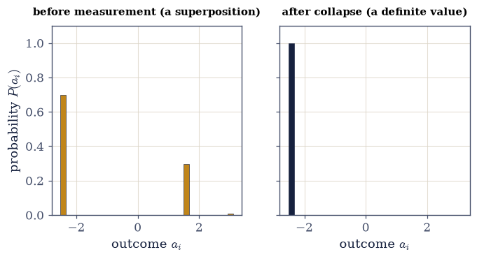
../../_images/a7e96350834c60fc415524673b3413b71c06ef847c485074917636b278ab340f.png — Fig. 519 **Collapse and repeatability.** *Left:* before measurement, the observable \(A\) has a spread of possible outcomes, each with its Born probability \(P(a_i)\) (amber) — the state is a genuine superposition with non-zero variance. *Right:* a measurement returns one eigenvalue and **collapses** the state onto that eigenspace; the very same observable, re-measured, now yields that value with probability one (ink) — a single definite outcome, zero variance. The collapse is Postulate 4, and the certainty of the repeat is *repeatability*, the property that lets “the system has this value now” mean something (the sequential Stern–Gerlach experiment of §6.4, made formal).#

Notebook summary#

Quantum mechanics, stated as five postulates — each the distilled content of a Stern–Gerlach fact, each in the language of Movement 0.

State Eq. 514: a unit vector \(|\psi\rangle\), a ray (§6.1).
Observable Eq. 515: a Hermitian \(A\), eigenvalues the outcomes, eigenvectors the definite-value states (§6.2).
Born rule Eq. 516: \(P(a_i)=|\langle a_i|\psi\rangle|^2=\langle\psi|P_i|\psi\rangle= \|P_i\psi\|^2\), the three forms agreeing and summing to one (§6.3).
Collapse Eq. 517: \(|\psi\rangle\to P_i|\psi\rangle/\|P_i|\psi\rangle\|\), repeatable — and onto the whole eigenspace when degenerate (the Lüders rule).
Dynamics Eq. 518: \(i\hbar\,\partial_t|\psi\rangle=H|\psi\rangle\) — stated here, worked out in §6.7.
Expectation and variance Eq. 519, Eq. 520: \(\langle A\rangle=\langle\psi| A|\psi\rangle=\sum_i a_iP(a_i)\) and \((\Delta A)^2=\langle A^2\rangle-\langle A\rangle^2\ge0\), zero on eigenstates — the laboratory’s mean and spread (§5.2, quantum).

We did not invent the postulates; the experiment forced them and Movement 0 named them. From five short rules — all met already in one experiment — the rest of the volume follows by computation.

Outlook#

Incompatible observables and the uncertainty relation (§6.6): commutators, when two observables cannot be simultaneously definite, and how much \(\Delta A\,\Delta B\) must exceed.
The dynamics postulate worked out (§6.7): the Schrödinger equation, the time-evolution operator \(U(t)=e^{-iHt/\hbar}\), spin precession and Rabi oscillations.
The Bloch sphere (§6.8): the geometry of qubit states and measurements.
Mixed states and the density matrix (§6.26): where “unit vector” generalizes to a density operator.
Cross-reference §6.1 (states), §6.2 (observables), §6.3 (projectors), §6.4 (the experiment), §5.2 (expectation/variance), and forward to §6.6, §6.7, §6.8, §6.26.

Take this notebook with you

Use the download button (↓) in the toolbar above to save this notebook and run it yourself. The published notebooks ship without worked solutions; if you would like the reference solutions — to teach from or to check your own work — get in touch: hello@ramador.me.